Programming video games, as many areas of science and technology, requires computing the coordinates of an object in different reference systems, constructed by combining together translations, rotations or scale changes.
The problem is particularly complex with the rotations. In a previous article we have studied the representation of rotations by means of matrices, highlighting their advantages and even their limitations.
The Euler angles were introduced by the great mathematician Euler (1707-1783) to study the rotational motion of a rigid body in the three-dimensional Euclidean space. The quaternions are algebraic structures, introduced by Hamilton (1805-1865), which extend the concept of complex numbers. Although they are less intuitive than Euler angles, they have proved to be a more efficient tool for studying the rotational motion of bodies. In this article, we’ll describe the properties of these two important topics and we’ll refer to their use in the Unity 3D framework.
1) Euler angles
1.1) Euler’s rotation theorem
Each displacement of a rigid body in three-dimensional space, with a point that remains fixed, is equivalent to a single rotation of the body around an axis passing through the fixed point.
This theorem was formulated by Euler in 1775. Given a rigid body with a fixed point, which initially is in a configuration \(C_ {0}\) and after a time interval \(t\) is in a configuration \(C_ {t}\), the theorem states that we can always identify a rotation around an axis that connects these two configurations.
In other words, if we have two Cartesian reference systems \((x, y, z)\) and \((X, Y, Z)\) with the same origin but different orientation, we can always find an equivalent rotation around a fixed axis through the origin that will give the same configuration.
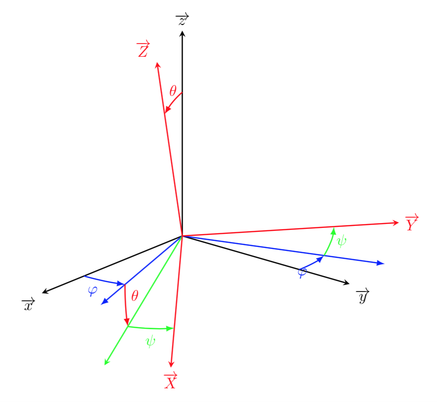
Each rotation can therefore be described by the three Euler angles, which specify a sequence of three successive rotations around the coordinate axes. The triplet of Euler angles is usually denoted with the notation \((\phi, \theta,\psi)\).
There are several conventions on how to express the angles of Euler, depending on the order of the rotations. Each of the three rotations can be performed around any coordinate axis. There are therefore several possible sequences, of length \(3\), to completely define the state of rotation of an object.
We use the convention associated with the \(ZYZ\) angles characterized by the following operations:
- Rotation of an angle \(\phi \) around the \(z\) axis
- Rotation of an angle \(\theta\) around the (current) \(y\) axis
- Rotation of an angle \(\psi\) around the \(z\) (current) axis
Each of the three rotations can be mathematically represented by a rotation matrix. The matrix relative to the overall rotation is calculated by multiplying the 3 matrices in the reverse order.
For a review of the representation of rotations by matrices see the article in this blog.
For a rotation around the axis \(Z\) of an angle \(\phi\):
For a rotation around the axis \(Y\) of an angle \(\theta\):
\[ \left( \begin{array}{cccc} \cos \theta & 0 & \sin \theta & 0 \\ 0 & 1 & 0 & 0 \\ -\sin \theta & 0 & \cos \theta & 0 \\ 0 & 0 & 0 & 1 \end{array} \right) \]For a rotation around the axis \(Z\) of an angle \(\psi\):
\[ \left( \begin{array}{cccc} \cos \psi & -\sin \psi & 0 & 0 \\ \sin \psi & \cos \psi & 0 & 0 \\ 0 & 0 & 1 & 0 \\ 0 & 0 & 0 & 1 \end{array} \right) \]Then, by multiplying in the reverse order we get the matrix relative to the overall rotation:
\[ \begin{array}{l} Rot(z,\psi)Rot(y,\theta)Rot(z,\phi)= \\ \left( \begin{array}{cccc} \cos \psi & -\sin \psi & 0 & 0 \\ \sin \psi & \cos \psi & 0 & 0 \\ 0 & 0 & 1 & 0 \\ 0 & 0 & 0 & 1 \end{array} \right) \cdot \left( \begin{array}{cccc} \cos \theta & 0 & \sin \theta & 0 \\ 0 & 1 & 0 & 0 \\ -\sin \theta & 0 & \cos \theta & 0 \\ 0 & 0 & 0 & 1 \end{array} \right) \cdot \left( \begin{array}{cccc} \cos \phi & -\sin \phi & 0 & 0 \\ \sin \phi & \cos \phi & 0 & 0 \\ 0 & 0 & 1 & 0 \\ 0 & 0 & 0 & 1 \end{array} \right) \\ \end{array} \]Given the rotation matrix \(Rot (z, \psi) Rot (y, \theta) Rot (z, \phi)\), it is possible to determine the corresponding Euler angles. Without going into the mathematical details, let us remember, however, that the conversion process is quite delicate. This is due to the possibility of having two different sequences for the same final orientation and also for the presence of degenerate cases, in the case of particular values of the angles.
1.2) Limits of the Euler angles
The Euler angles have the characteristic of simplicity, are easy to understand and require only \(3\) real floating point numbers.
Unfortunately, they suffer from a problem called Gimbal Lock. Applying the rotations in sequence it can happen that one of the three main axes collapses in one of the other two. For example, if we rotate \(90\) degrees around the \(X\) axis, the \(Y\) axis will collapse on the \(Z\) axis. In this situation a degree of freedom is lost as the rotations around the \(Y, Z\) axes become equivalent.
Another drawback is that the angles depend on the order of the three rotations, represented with the indication of the rotation axes: \(ZYZ, XZX, YXY\), etc. Each combination gives a different result, as is easy to verify.
Despite these problems, the Euler angles are commonly used in many areas, including CAD modeling tools and video game development frameworks. For example, the Unity 3D interface in the Inspector panel displays the Euler angles to represent the rotation state of a game object. However, within the programs responsible for the calculations to simulate rotations, Unity uses a much more powerful mathematical tool, represented by Hamilton’s quaternions.
2) Hamilton’s quaternions
The quaternions were introduced by Hamilton as a four-dimensional extension of complex numbers. These new mathematical objects have provided a powerful tool to perform the complex calculations needed to study rotations in three-dimensional space.
For an understanding of the quaternion algebra it’s necessary to know the fundamentals of vector calculus in Euclidean space \(R ^{3}\). For this you can consult the following texts: [1], [2].
Quaternions can be considered as extensions of complex numbers. As is known, a complex number \(z\) is written with the notation \(z = a + bi\), where \(i\) is the imaginary unit defined by \(i ^ 2 = -1\). To define a quaternion \(\mathbf {q}\) we add two more symbols \(j, k\):
\[ \mathbf{q} = w + xi + yj + zk \]where \(w\) is the real part, \((i, j, k)\) denote the three imaginary units, and \((x, y, z)\) denote the three imaginary components.
It’s convenient to use an abbreviated notation to represent a quaternion
where \(w\) is the scalar component and \(\mathbf {v} = (x, y , z)\) is the vector with the imaginary components \((x, y, z)\). We’ll denote the algebraic structure of the quaternions with the symbol \(\mathbb {H}\). The quaternion algebra is based on the following rules introduced by Hamilton:
\[ i^{2}=j^{2}=k^{2}=ijk=-1 \] \[ ij=k=-ji \] \[ jk=i=-kj \] \[ ki=j=-ik \]2.1) Addition and multiplication of quaternions
Given two quaternions
\[ \begin{array}{l} \mathbf{q}_{1}= w_{1} + x_{1}i + y_{1}j + z_{1}k \\ \mathbf{q}_{2}= w_{2} + x_{2}i + y_{2}j + z_{2}k \\ \end{array} \]the sum is defined as
\[ \mathbf{q}_{1} + \mathbf{q}_{2}= (w_{1}+w_{2}) + (x_{1} + x_{2}) i + (y_{1}+y_{2})j + (z_{1}+z_{2})k \]while the product of the two quaternions is defined as follows:
\[ \begin{array}{l} \mathbf{q}_{1} \mathbf{q}_{2} =& (w_{1}w_{2} – x_{1}x_{2}-y_{1}y_{2}-z_{1}z_{2}) \\ &+ \ (w_{1}x_{2} + x_{1}w_{2}+ y_{1}z_{2}-z_{1}y_{2})i \\ &+ \ (w_{1}y_{2} – x_{1}z_{2}+ y_{1}w_{2}+z_{1}x_{2})j \\ &+ \ (w_{1}z_{2} + x_{1}y_{2}- y_{1}x_{2} +z_{1}w_{2})k \\ \end{array} \]A more concise notation of the product is obtained if we use
the notation \(\mathbf{q}_{1}= w_{1}+ \mathbf{v_{1}}\) and \(\mathbf{q}_{2}= w_{2}+ \mathbf{v_{2}}\):
where \(\mathbf {v_ {1}} \bullet \mathbf {v_ {2}}\) is the scalar product of the two vectors and \(\mathbf {v_ {1}} \times \mathbf {v_ {2} }\) is the vector product.
2.2) Conjugate, standard and inverse of a quaternion
The conjugate of a quaternion \(\mathbf {q}\) is a quaternion denoted by \(\mathbf {q} ^ {*}\) so defined:
\[ \mathbf{q}^* = q_0 – q_1 i – q_2 j – q_3 k \]By multiplying a quaternion with its conjugate we have:
\[ \mathbf{q} \mathbf{q}^* = (q_0 + \mathbf{v})(q_0 – \mathbf{v}) = q_0^2 + q_1^2 + q_2^2 + q_3^2 \]The length, or norm, of a quaternion \(\mathbf {q}\) is so defined:
\[ N(\mathbf{q})=\left\|\mathbf{q}\right\| = \sqrt{\mathbf{q} \mathbf { q}^*} = \sqrt{q_0^2 + q_1^2 + q_2^2 + q_3^2} \]Each quaternion, with the exception of zero, has an inverse with respect to the product:
\[ \mathbf{q}^{-1} = \frac{\mathbf{q}^*}{\left\|\mathbf{q}\right\|^2} \]To carry out the division between two quaternions it’s enough to multiply the first by the inverse of the second.
Thanks to the properties illustrated above we can conclude that, while complex numbers constitute an algebraic field, quaternions are a division ring, since the commutative property of the product doesn’t hold for them. Moreover, the quaternions have a vector space structure of dimension 4 on the field of real numbers.
The disadvantage of quaternions is that they are less intuitive to humans than Euler angles. However, their characteristics make them indispensable for computations performed through software programs.
Exercise 2.1
Given a quaternion \(\mathbf {q} = q_ {0} + i q_ {1} + jq_ {2} + kq_ {3}\), show that the following formula holds:
Exercise 2.2
Given two quaternions \(a, b \in \mathbb {H}\), prove the following formula:
Exercise 2.3
Compute the quotient of the two quaternions \(\mathbf{q}_{1}= 2 + i + 3j -k\) and \(\mathbf{q}_{2}=-1 +2i +j -4k\).
Answer
3) Quaternions and rotations
As is known, a rotation in three-dimensional space is a function \(\psi \colon \mathbb {R} ^ {3} \to \mathbb {R} ^ {3}\) that preserves lengths, angles and orientation. The following relations must be respected:
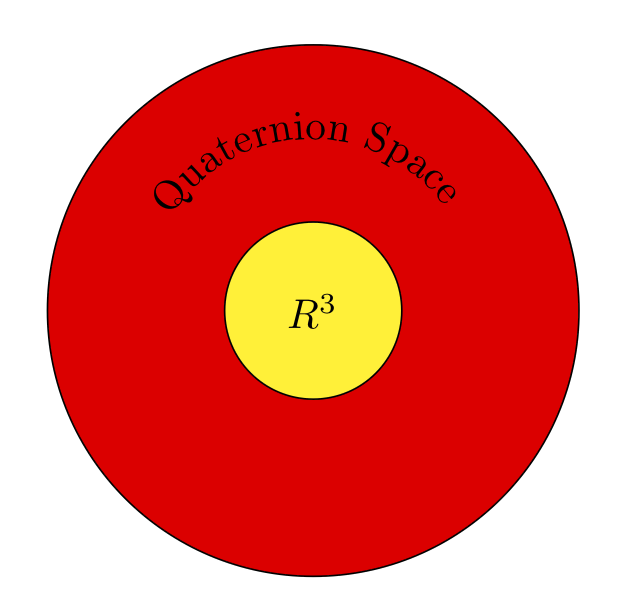
\[ \begin{split} \left\| \psi (\mathbf{P}) \right\| &= \left\|\mathbf{P} \right\| \\ \psi (\mathbf{P}_{1}) \bullet \psi (\mathbf{P}_{2}) &= \mathbf{P}_{1} \bullet \mathbf{P}_{2} \\ \psi (\mathbf{P}_{1}) \times \psi (\mathbf{P}_{2}) &= \psi (\mathbf{P}_{1} \times \mathbf{P}_{2}) \end{split} \]where the symbol \(\bullet\) denotes the scalar product of two vectors, and the symbol \(\times\) denotes the vector product. We use the symbol \(Im (\mathbb{H})\) for the set of quaternions with the scalar component equal to zero. The quaternions belonging to the space \(Im (\mathbb {H})\) are called imaginary or pure quaternions.
We can then identify \(Im(\mathbb {H})\) with the three-dimensional space \(\mathbb{R}^ {3}\). It follows that, given two imaginary quaternions \(\mathbf {P}_{1}, \mathbf {P}_{2}\), their product is given by the formula:
Theorem 3.1
Let \(\psi\) be a rotation in the space \(\mathbb{R}^{3}\). We define a new function \(\Psi\), extension of the \(\psi\) in the space \(\mathbb{H}\) with this condition:
Then the following relationship applies:
\[ \Psi (\mathbf{P}_{1}\mathbf{P}_{2})=\Psi(\mathbf{P}_{1}) \Psi(\mathbf{P}_{2}) \]where \(\mathbf{P}_{1}, \mathbf{P}_{2}\) are pure quaternions with zero scalar part. We say that the function \(\Psi\) is a homomorphism in the space \(\mathbb{H}\).
Proof
Just apply the product formula of two imaginary quaternions and the properties of the operator \(\psi\) applied to the space vectors \(\mathbf {R} ^ {3}\).
According to the previous theorem, functions such as \(\Psi\) represent rotations in three-dimensional space.
We now define a class of functions \(\Psi_{\mathbf{q}}(\mathbf {P}) = \mathbf{q}\mathbf{P}\mathbf{q}^{- 1}\). It’s easily proved that this transformation respects the invariance of the norm and is a homomorphism in space \(\mathbb {H}\). It’s enough to apply the definition of the function and remember that
Thus each quaternion can be associated with the rotation of an angle \(\theta\) around an axis \(\mathbf {v}\). To find the correspondence formula, it’s convenient to study the properties of unity quaternions.
4) Unit quaternions
If \(\left\| \mathbf{q} \right\| =1\) then \(\mathbf {q}\) it is called a unity quaternion.
Theorem 4.1
A unity quaternion can be represented in the form
Proof
If \( \left\| \mathbf{q} \right\|=1\) and \(\mathbf {q} = (w, (x, y, z))\), then \(w ^ {2 } + x ^ {2} + y ^ {2} + z ^ {2} = 1\). Because \(w ^ {2} <1\), we can assume that \(w = \cos \theta\) for some angle \(\theta\).
From the trigonometric identity \(\sin ^ {2} \theta + \cos ^ {2}\theta = 1\) we derives \(x ^ {2} + y ^ {2} + z ^ {2} = \sin ^ {2}\theta\). So \(\mathbf {v}\) is a unit vector \((\frac {x} {r}, \frac {y} {r}, \frac {z} {r})\) with \(r = \sqrt {x ^ {2} + y ^ {2} + z ^ {2}}\).
The conjugate of a unity quaternion \(\mathbf{q}=(\cos \theta, \mathbf{v} \sin \theta)\) can be written as
\[ \mathbf{q}^{*}= (\cos \theta, -\mathbf{v} \sin \theta)=(\cos (-\theta), \mathbf{v} \sin (-\theta)) \]The product of two unity quaternions is a unity quaternion:
\[\left\| \mathbf{q}_{1} \mathbf{q}_{2} \right\| = \left\|\mathbf{q}_{1} \right\| \left\|\mathbf {q}_{2}\right\|=1 \]Theorem 4.2
The inverse of a unity quaternion is the conjugate quaternion, and it’s a unity quaternion.
Proof
The theorem follows directly from the properties of the conjugate. However, it is useful to have confirmation also by performing the product with the trigonometric representations:
5) Unit quaternions represent rotations
To represent a rotation in space we need a unit vector \(\mathbf {u}\), in the direction of the rotation axis, and an angle \(\theta\) which tells us the value of the rotation. Then we indicate with \(R (\theta, \mathbf {v})\) the operator that, applied to a vector \(\mathbf {v}\), gives as a result the new position of the vector after the rotation.
To calculate the value of \(R (\theta, \mathbf {v})\), first the vector is decomposed into its components, parallel and orthogonal to the rotation axis:
It can be shown that the following formula is valid, regarding the resultant vector after the rotation of a vector \(\mathbf {v}\) by an angle \(\theta\) around an axis \(\mathbf {u}\) :
\[ \begin{array}{l} R(\mathbf{v},\theta)= R (\mathbf{v}_{p},\theta) + R(\mathbf{v}_{o},\theta)= \\ (\cos \theta) \mathbf{v} + (1 – \cos \theta) \mathbf{u} (\mathbf{u} \bullet \mathbf{v}) + (\sin \theta)(\mathbf{u} \times \mathbf{v}) \end{array} \]For a proof, in addition to the texts cited in the bibliography, you can see the following link to Wolfram.
On the other hand, given a pure quaternion \(\mathbf {P} = (0, \mathbf {v})\) and a unity quaternion \(\mathbf {q} = (\cos \theta, \mathbf {u} \sin\theta)\) the following formula applies:
\[ \begin{split} \mathbf{q} \mathbf{P} \mathbf{q}^{*} =\ & (\cos \phi, \mathbf{u} \sin \phi)(0,\mathbf{v})(\cos \phi, -\mathbf{u} \sin \phi) = \\ & (0,(\cos ^{2} \phi-\sin^{2} \phi)\mathbf{v} + 2 \sin^{2} \phi(\mathbf{u} \bullet \mathbf{v}) \mathbf{u} + \\ & \ 2 \sin \phi \cos \phi (\mathbf{u} \times \mathbf{v})) = \\ & (0,(cos 2\phi)\mathbf{v}+ (1- \cos 2\phi)(\mathbf{u} \bullet \mathbf{v}) \mathbf{u} + (\sin 2\phi)(\mathbf{u} \times \mathbf{v})) \end{split} \]By comparing the last two equations, we can conclude that they are equivalent, with the substitution \(\theta = 2 \phi\).
Another way to reach the same result is the following. Let \(\mathbf {q} = w + \mathbf {u}\) be a unity quaternion. The inverse of \(\mathbf {q}\) is \(\mathbf {q} ^ {- 1} = \mathbf {q} ^ {*} = w- \mathbf {u}\). Given an imaginary quaternion \(\mathbf {P} = (0, \mathbf {v})\), we have
Now we make use of the following known properties of vector calculus:
\[ \mathbf{v} \times (\mathbf{u} \times \mathbf{v}) = \mathbf{v} \times \mathbf{u} \times \mathbf{v}= v^{2}\mathbf{u}-(\mathbf{v} \bullet \mathbf{u})\mathbf{v} \]Then we can write:
\[ \mathbf{q} \mathbf{P} \mathbf{q}^{-1}= (w^{2} – \mathbf{u}^{2})\mathbf{P}+ 2w \mathbf{u} \times \mathbf{P}+ 2(\mathbf{u} \bullet \mathbf{P})\mathbf{u} \]Set \(\mathbf {u} = t\mathbf {A}\), where \(\mathbf {A}\) is a unit vector, we have:
\[ \mathbf{q} \mathbf{P} \mathbf{q}^{-1}=(w^{2} – t^{2})\mathbf{P} + 2wt \mathbf{A} \times \mathbf{P}+ 2 t^{2}(\mathbf{A} \bullet \mathbf{P}) \mathbf{A} \]Comparing with the rotation formula in three-dimensional space written around an arbitrary axis, we have the following relationships:
\[ \begin{align} w^{2} – t^{2} &= \cos \theta \\ 2 w t &= \sin \theta \\ 2t^{2} &= 1 – \cos \theta \end{align} \]With a few steps, we can deduce the following formulas:
\[ w=\cos \left (\frac{\theta}{2}\right) \quad t=\sin\left(\frac{\theta}{2}\right) \]So the unitary quaternion that corresponds to a rotation around the axis \(\mathbf {A}\) is:
\[ \mathbf{q} = \cos \left (\frac{\theta}{2}\right) +\mathbf{A} \sin \left(\frac{\theta}{2}\right); \]The product of two quaternions \(\mathbf {q}_{1}, \mathbf {q}_{2}\) represents the rotation resulting from the composition of the two individual rotations.
5.1) Rotation matrix corresponding to a quaternion
To calculate the matrix corresponding to a quaternion, just expand the formula:
\[ \mathbf{q} \mathbf{P} \mathbf{q}^{-1}=(w^{2} – t^{2})\mathbf{P} + 2wt \mathbf{A} \times \mathbf{P}+ 2 t^{2}(\mathbf{A} \bullet \mathbf{P}) \mathbf{A} \]The result is the following matrix \(M\):
\[ \left( \begin{array}{ccc} 1-2y^{2}- 2z^{2} & 2xy -2wz & 2xz+2wy \\ 2xy+2wz & 1-2x^{2}-2z^{2} & 2yz-2wx \\ 2xz-2wy & 2yz+2wx & 1-2x^{2}-2y^{2} \\ \end{array} \right) \]Given the rotation matrix described above, it’s possible to find the corresponding quaternion with a few passages. First we compute the trace of the matrix \(M\) (sum of diagonal elements)
\[ Tr(M)= 3-4x^{2}-4y^{2}-4z^{2}=4w^{2}-1 \]since the quaternion is unitary \((x ^ {2} + y ^ {2} + z ^ {2} + w ^ {2} = 1)\). So we have
\[ w=\sqrt {\frac{Tr(M)+1}{4}} \]In the same way we compute the other components \(x, y, z\).
6) Rotations in Unity 3D
6.1) The Transform component
Each Unity object, even if it’s not visible on the scene, has the Transform component, which contains very important information about the object to which it’s associated. Among these we remember position, rotation and scale factor. Virtually, the Transform component consists of a matrix that stores information about position, rotation and scale.
6.2) Rotations
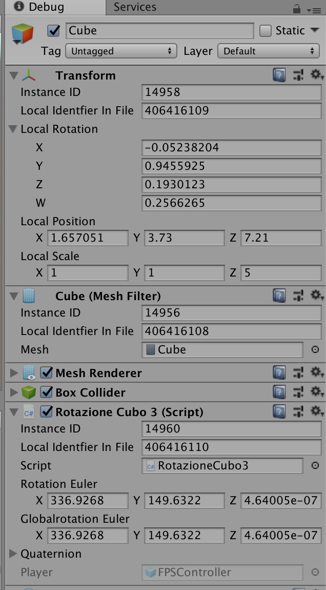
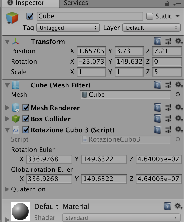
The Unity editor uses vectors and Euler angles to represent the position and direction of an object, while internally the engine uses quaternions for complex calculations. The Transform component displays the values of the Euler angles if the editor is in normal mode, while in debug mode it displays the components \((W, X, Y, Z)\) of the quaternion.
Unity provides many functions that connect vectors, Euler angles and quaternions. Let’s have a look at some examples:
 // Create a quaternion to represent a rotation of 40
// degrees around the X-axis, 15 around the X-axis and 10
// around the Y-axis (in the order ZXY)
Quaternion q1 = Quaternion.Euler(40, 15, 10);

//Create a quaternion from Euler angles
Vector3 rotEulero = new Vector3(40, 15, 10);
Quaternion q2 = Quaternion.Euler(rotEulero);

// Convert quaternions to Euler angles
Quaternion q3 = transform.rotation;
Vector3 euler = q3.eulerAngles;
Debug.Log("Euler angles x: euler.x + " y: " euler.y +
" z: " + euler.z);
Unity provides various options like Vector3.right, back, forward, down, up, left, right. For example, to rotate in the negative direction of the horizontal axis use Vector.left, which is equivalent to \((-1,0,0)\).
Among the main functions made available by Unity we recall the following, for which we refer to the online Unity 3D documentation:
- Quaternion.LookRotation
- Quaternion.Angle
- Quaternion.Euler
- Quaternion.Slerp
- Quaternion.FromToRotation
- Quaternion.identity
Example 6.1
Rotation around the \(X\) axis by one degree per second:
void Update() {
     transform.Rotate(Vector3.left * Time.deltaTime);
}
Example 6.2
Rotation to track a Target object:
// Find object with id = "Target"
public Transform target = GameObject.Find("Target").GetComponent<Transform>();

// Compute difference position vector
Vector3 vectorDiff = target.position - transform.position;

// Create rotation
Quaternion rotation = Quaternion.LookRotation(vectorDiff);

// Set rotation property of transform component
transform.rotation = rotation;
Conclusion
The Euler angles and Hamilton’s quaternions are two very important methods for representing the rotations of objects in three-dimensional space. The Euler angles, despite being more intuitive, suffer from the gimbal lock problem. Quaternions do not have a simple physical interpretation. However they are preferred for performing complex calculations, because they have a compact representation, do not have the gimbal lock problem and have other advantages, among which for example:
- simplicity to represent the composition of two rotations through the product of quaternions
- spherical linear interpolation, with which it’s possible to generate intermediate orientations between two states of rotations, obtaining a fluid animation
The most advanced properties of the quaternions will be the subject of a later study. For further information, see the book by Van Verth and Bishop[3].
Bibliography
[1]Murray, Spiegel – Vector Analysis (McGraw-Hill)
[2]H. Goldstein – Classical Mechanics (Pearson)
[3]Van Verth, Bishop – Essential Mathematics for Games and Interactive Applications (AK Peters)

0 Comments