1) Algebra of matrices
A matrix \(A(m,n)\) defined on the field of real numbers \(\mathbb{R}\) is a collection of real numbers \((a_{ij})\), indexed by natural numbers \(i, j\), with \(1\le i\le m\) and \( 1\le j\le n\). We can represent a matrix with a rectangular array of numbers arranged in \(m\) rows and \(n\) columns:
\[ \begin{pmatrix} a_{11} & a_{12} & \cdots & a_{1n} \\ a_{21} & a_{22} & \cdots & a_{2n} \\ \vdots & & \ddots & \vdots \\ a_{m1} & a_{m2} & \cdots & a_{mn} \\ \end{pmatrix} \]A column vector is a matrix \(m\times 1\) for some \(m\), while a row vector is a matrix \(1\times n\) for some \(n\). The symbol \(\mathbb{R}^{m\times n}\) it is used to represent the set of all matrices \(m\times n\) with real coefficients.
Matrix definitions and operations can be extended similarly in the field of complex numbers \(\mathbb{C}\).
Given two matrices of the same order, we can define addition and subtraction operations:
Given a matrix \(A(m,p)\) and a matrix \(B(p,n)\), then it is possible to define the product of the two matrices, which results in a new matrix \(C(m,n)\), whose elements \(c_{ij}\) are
\[ c_{ij} = \displaystyle\sum_{k=1}^{p} a_{ik}b_{kj} \qquad 1\le i\le m \quad 1\le j\le n \]If \( \lambda \in \mathbb{R} \) and \(A\) is a matrix with coefficients \(a_{ij}\), then we indicate with \(\lambda A\) the matrix whose coefficients are equal to \(\lambda a_{ij}\).
The identity matrix of order \(n\), indicated with \(I_n\), is defined as follows:
Given a matrix \(A(n,n)\), the matrix \(B(n,n)\) is called the inverse of \(A\) if \(AB=I_{n}\). The matrix obtained by exchanging the rows with the columns of the matrix A it is called the transpose of A, and is indicated with the symbol \(A^{T}\).
Given the matrices A, B, and C and a real number \(\lambda\), the following properties are easily proved:
For a square matrix it is possible to define and compute the determinant, which is a scalar, that is a real number. For the identity matrix \(I_{n}\) we have \( det(I_{{n}})=1\). For a square matrix \(A(2,2)\), the calculation is simple:
\[ det(A) = det \begin{pmatrix} a_{11} & a_{12} \\ a_{21} & a_{22} \\ \end{pmatrix} = a_{11} a_{22} – a_{12} a_{21} \]For a matrix \(A(3,3)\) the calculation is more complex; the following diagram, which illustrates Sarrus’ rule, can be useful:
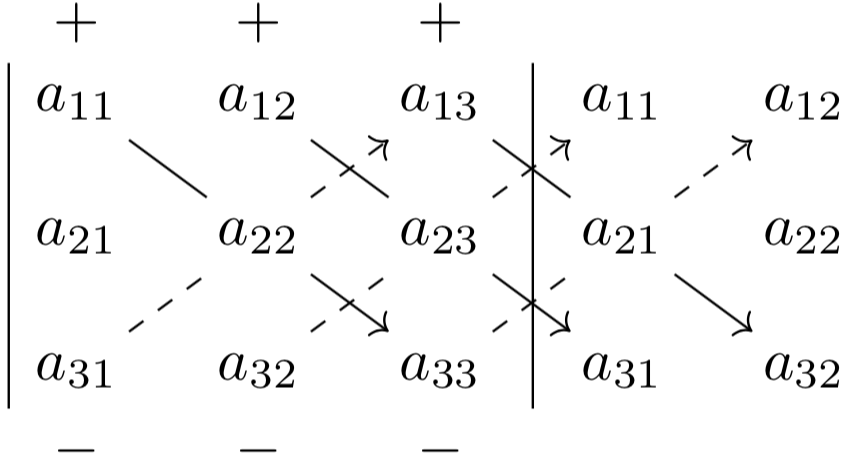
So the determinant of a matrix \(A(3,3)\) is:
\[ \begin{array}{l} det(A)= a_{11}a_{22}a_{33}+ a_{12}a_{23}a_{31}+ a_{13}a_{21}a_{32}- \\ a_{13}a_{22}a_{31}- a_{11}a_{23}a_{32}- a_{12}a_{21}a_{33} \\ \end{array} \]The value of the determinant makes it possible to determine whether the rows or columns of a matrix are independent of each other.
It is also useful in solving systems of linear equations. A system of linear equations with \(m\) equations and \(n\) unknowns is defined by the following equations:
The system can be written in a compact form such as \(Ax = b\), where \(A\) is the matrix \(m\times n\) with coefficients \(a_{ij}\), \(x\) is the column vector with coefficients \(x_i\), and \(b\) is the column vector with coefficients \(b_i\).
For an in-depth study of matrix operations, determinants and systems of linear equations, see for example [1].
2) Linear transformations
Matrices are often used to transform an object from one space to another. A linear transformation is a function
\[ T: \mathbb{R}^{n} \to \mathbb{R}^{m} \]such that for all \(x,y\in \mathbb{R}^{n}\) and \( \lambda\in \mathbb{R}\) :
\[ T(x+y) = T(x) + T(y) \quad T(\lambda x) = \lambda T(x) \]If \(T:\mathbb{R}^{n} \to \mathbb {R}^{m}\) is a linear transformation, \(x_1,\ldots,x_k\in \mathbb{R}^{n}\), and
\( \lambda_1,\ldots,\lambda_k\in \mathbb {R}\), then:
If \( \lambda \in \mathbb{R}\) and \( S, T : \mathbb {R}^{n} \to \mathbb {R}^{m}\) are two linear transformations, so are the following ones \(S + T\) and \(\lambda T\):
\[ \begin{array}{l} (S + T)(x) = S(x) + T(x) \quad x\in \mathbb {R}^{n}\\ \\ (\lambda T)(x) = \lambda (T(x)) \quad x\in \mathbb {R}^{n} \\ \end{array} \]Every linear transformation \(T\) can be represented by a matrix \(A\), and vice versa every matrix represents a linear transformation, through the relation \(T(x) = Ax\), where the symbol \(Ax\) means the product of the matrix \(A\) by the vector \(x\).
3) Orthogonal transformations and orthogonal matrices
Let us recall the definition of scalar product \(x \cdot y\) of two vectors \(x,y \in \mathbb{R}^{n}\) :
\[ x\cdot y = x_{1}y_{1} + x_{2}y_{2} + … + x_{n}y_{n} \]The norm of a vector \(x\), indicated with the symbol \({\left\| {x}\right\|}\), can be computed using the Pythagorean Theorem:
\[ {\left\| {x}\right\|}=\sqrt{x_{1}^{2} + x_{2}^{2} + \cdots +x_{n}^{2}} \]An orthogonal transformation is a linear transformation that preserves the scalar product of the vectors and therefore preserves the distance between two points. In formulas we have:
\[ \begin{array}{l} T(x) \cdot T(y) = x \cdot y \\ \\ \Vert T(x) – T(y)\Vert = \Vert x- y\Vert \\ \\ \Vert T(x) \Vert = \Vert x \Vert \\ \end{array} \]The matrix that represents an orthogonal transformation is called an orthogonal matrix and has the following properties:
\[ A^{T}A = I \quad A^{T} = A^{-1} \]that is, the transposed matrix coincides with the inverse matrix. Since the determinant of the transposed matrix of \(A\) is equal to that of the original matrix, we have:
\[ det (A) \times det (A^{T}) = det (I) = 1 \quad \implies det (A) = \pm 1 \]We can have two distinct cases:
- \( det (A) = +1\) : the matrix represents a rotation
- \( det (A) = -1\) : the matrix represents a reflection
In the plane a rotation of an angle \( \theta\) is represented by an orthogonal matrix \(A\) with \( det (A) = +1\) :
\[ A = \left( \begin{array}{cc} \cos \theta & -\sin \theta \\ \sin \theta & \cos \theta \\ \end{array} \right) \]An example of reflection in the plan (\(det (A) = -1\)) is the following:
\[ A = \left( \begin{array}{cc} \cos \theta & \sin \theta \\ \sin \theta & -\cos \theta \end{array} \right) \]4) 4×4 matrices and homogeneous coordinates
A fundamental requirement in video games is being able to represent the position of objects, the state of rotation and the scale factor of the three dimensions.
The homogeneous coordinates allow to represent all this information with a single object, a 4×4 matrix. Four homogeneous coordinates are used to represent the state of an object in a 3D environment. You can use an orthonormal matrix for the rotation and, through the homogeneous coordinates, expand the matrix from 3×3 to 4×4 to add the information on the position and the scale.
We use the notation (x, y, z, w) for the vectors, with the following conventions:
- if w = 1, then the vector (x,y,z,1) represents the position in space
- if w = 0, then the vector (x,y,z,0) represents a direction
Translation matrices
A translation matrix has the following structure:
\[ \left( \begin{array}{cccc} 1 & 0 & 0 & X \\ 0 & 1 & 0 & Y \\ 0 & 0 & 1 & Z \\ 0 & 0 & 0 & 1 \end{array} \right) \]
where \(X,Y,Z\) are the values we want to add to the position.
Matrices for scale change
The parameters for scale change are stored in the diagonal. The matrices have the following structure:
\[ \left( \begin{array}{cccc} x & 0 & 0 & 0 \\ 0 & y & 0 & 0 \\ 0 & 0 & z & 0 \\ 0 & 0 & 0 & 1 \end{array} \right) \]For example if you want to scale a vector of \(3\) units in all directions, the matrix is:
\[ \left( \begin{array}{cccc} 3 & 0 & 0 & 0 \\ 0 & 3 & 0 & 0 \\ 0 & 0 & 3 & 0 \\ 0 & 0 & 0 & 1 \end{array} \right) \cdot \left( \begin{array}{c} x \\ y \\ z \\ w \end{array} \right) = \left( \begin{array}{c} 3x \\ 3y \\ 3z \\ w \end{array}\right) \]while the coordinate w does not change.
Rotation matrices
A rotation in 3D space can be expressed by 3 successive single rotations, one around the X axis, another to the Y axis, and the last around the Z axis.
For a rotation around the x-axis of an angle \(\theta\) :
For a rotation around the y-axis of an angle \(\theta\) :
\[ \left( \begin{array}{cccc} \cos \theta & 0 & \sin \theta & 0 \\ 0 & 1 & 0 & 0 \\ -\sin \theta & 0 & \cos \theta & 0 \\ 0 & 0 & 0 & 1 \end{array} \right) \]For a rotation around the z-axis of an angle \(\theta\) :
\[ \left( \begin{array}{cccc} \cos \theta & -\sin \theta & 0 &0 \\ \sin \theta & \cos \theta & 0 & 0 \\ 0 & 0 & 1 & 0 \\ 0 & 0 & 0 & 1 \end{array} \right) \]A sequence of transformations (for example a translation followed by a rotation) is represented by a matrix that is determined by computing the product of the matrices corresponding to the elementary transformations. So to perform a scale change, a rotation and a translation of a vector, just multiply the 3 relative matrices in the opposite order:
TransformedVector = TranslationMatrix * RotationMatrix * ScaleMatrixExample: a 30-degree rotation is given around the x-axis followed by a translation (1,-1,2) along the x,y,z axes. The corresponding matrix is:
\[ \left( \begin{array}{cccc} 1 & 0 & 0 & 1 \\ 0 & 1 & 0 & -1 \\ 0 & 0 & 1 & 2 \\ 0 & 0 & 0 & 1 \end{array} \right)\cdot \left(\begin{array}{cccc} 1 & 0 & 0 & 0 \\ 0 & \cos \theta & -\sin \theta & 0\\ 0 & \sin \theta & \cos \theta & 0 \\ 0 & 0 & 0 & 1 \end{array} \right) = \left( \begin{array}{cccc} 1 & 0 & 0 & 1 \\ 0 & \cos \theta & -\sin \theta & -1\\ 0 & \sin \theta & \cos \theta & 2 \\ 0 & 0 & 0 & 1 \\ \end{array} \right) \]4.1) Disadvantages of using matrices to represent the rotations
Representing rotations with matrices has some drawbacks. First, 16 floating point numbers are needed to store data with 4 × 4 matrices. Rounding operations on floating point numbers cause a progressive loss of the orthogonality property of the matrices, with the consequence of having undesirable effects of deformations or contractions.
Other more efficient tools to represent and calculate the state of rotation of a 3D object are Euler angles and Hamilton Quaternions.
Euler’s theorem states that, if a rigid body with a fixed point go from an initial configuration \(C_{0}\) to a final \(C_{t}\) in a time interval \( t\), then we can determine an equivalent rotation around a fixed axis that transforms the initial position into the final one. Each rotation can then be described by the 3 Euler angles, which specify a sequence of 3 successive rotations around the Cartesian axes. The overall transformation can be represented with a matrix, obtained by multiplying together the matrices of the 3 single transformations.
The Unity framework, together with others, uses Euler angles and Hamilton Quaternions to represent rotations and perform calculations. These topics will be the subject of study in a future article.
5) Projection matrices
To visualize a scene on a 2D flat screen it’s necessary to perform a mathematical transformation called projection, which creates a 2D image of a 3D scene by projecting points or vertices making up the objects of the 3D scene onto the screen. There are two main types of projection:
- the perspective projection
- the orthographic projection
In the perspective projection the most distant objects appear smaller; parallel lines converge at a point called vanishing point, or point at infinity.
In the orthographic projection the objects appear of the same size, regardless of the distance from the camera. Parallel lines in 3D space remain parallel even in the projected image.
The type of projection to use depends of course on the type of game.
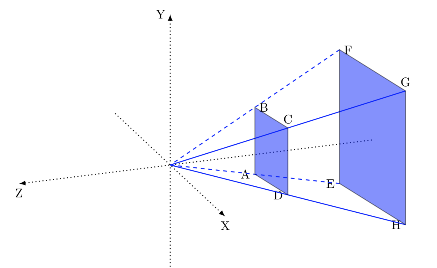
The volume that defines all the potentially visible points on the screen is called ‘view frustum‘. This volume depends on the camera eye arrangement. If the perspective projection is used, the shape of the frustum is a truncated pyramid. In the case of orthographic projection it is a rectangular prism. The vertex of the pyramid corresponds to the position of the camera and the base of the pyramid is called the far plane. To define the ‘view frustum’ two planes perpendicular to the Z axis are fixed:
- the far plane
- the near plane
This two planes delimit the visual field, which is therefore limited by the 6 surfaces of the pyramid trunk.
The fundamental problem to be solved is therefore to project the objects present in the area of the ‘view frustum’ on the screen of the device used for the game. From the mathematical point of view, therefore, the \(4 × 4\) matrix representing the perspective or orthographic projection must be determined.
In reality the transformation takes place in two phases:
- transformation of the points of the view frustum into a cube, called homogeneous clip space, an intermediate space independent of the type of projection used. The homogeneous coordinates of the intermediate space \( [x,y,z,w]\) are also normalized by dividing by \(w : [\frac{x}{w},\frac{y}{w},\frac{z}{w},\frac{w}{w}]\) (normalized device space or NDC).
- transformation of the clip space into the screen space
The determination of the transformation matrix allows to calculate the coordinates of the on-screen images of the objects that are inside the ‘view volume’. The calculation of the matrices that allow to carry out the two projections from the 3D scene on the 2D screen is quite complicated, and will be described in a next article. Here we limit ourselves to exposing the matrices.
Matrix for perspective projection
Based on the diagram of the ‘view frustum’ above, we define the coordinates of the various points:
\[ \{A=(l,b,-n); B=(l,t,-n); C=(r,t,-n); D=(r,b,-n) \} \] \[ \{E=(l,b,-f); F=(l,t,-f); G=(r,t,-f); H=(r,b,-f)\} \]where the symbols have the following meaning:
\[ \{l=left, r=right, b=bottom, t=top, n=near, f=far\} \]The matrix for the perspective projection is the following:
\[ \left( \begin{array}{cccc} \frac{2n}{r-l} & 0 & \frac{r+l}{r-l} & 0 \\ 0 &\frac{2n}{t-b} &\frac{t+b}{t-b }& 0 \\ 0 & 0 & \frac{f+n}{f-n} & \frac{2nf}{f-n} \\ 0 & 0 & -1 & 0 \end{array} \right) \]Matrix for orthographic projection
With the same notations for points, we have the following matrix:
\[ \left( \begin{array}{cccc} \frac{2}{r-l} & 0 & 0 & -\frac{r+l}{r-l}; \\ 0 &\frac{2}{t-b} & 0 &-\frac{t+b}{t-b }\\ 0 & 0 & \frac{-2}{f-n} & -\frac{f+n}{f-n} \\ 0 & 0 & 0 & 1 \end{array} \right) \]For an in-depth study of the matrices used in the projections, see for example [2].
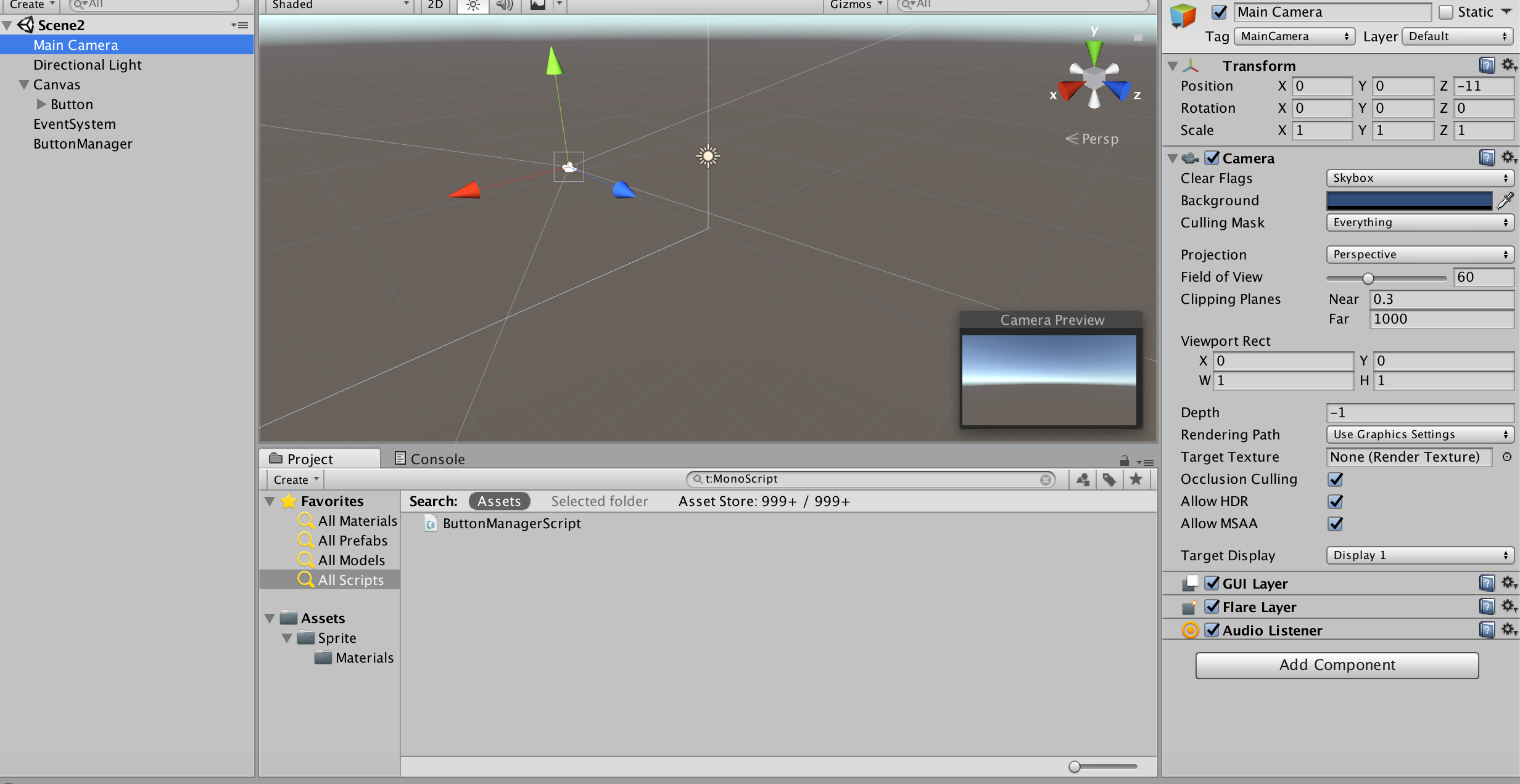
6) Matrices and systems of coordinates in Unity
To specify the position of an object in space it is first necessary to define a reference system (for example a Cartesian reference). So for each object the position is determined by its three coordinates relative to the reference system.
There are different types of reference spaces in Unity: global space (world space), local space, camera space, screen space and viewport. In each space a coordinate system is defined to describe the position of each object.
In the global space the coordinates of each object are referred to a fixed point, the origin. Local space is defined relative to an object: the origin is the center of the object, which naturally can be in motion, and the vertices of the object are defined with respect to this local origin. In the camera space the coordinates are referred to the position of the camera, and therefore of the observer. In the screen space a coordinate system is defined to identify each point on the screen (coordinate UI), taking as its origin \((0,0\)) the bottom left corner. The Viewport has a normalized coordinate system, with coordinates \((0,0)\) for the lower left point, and the coordinates \((1,1)\) for the point at the top right.
The Unity Transform component contains very important information for each object (GameObject) to which it belongs, including:
- position – the position of the gameObject (expressed with a Vector3)
- rotation – rotation (expressed as Quaternion)
- scale – the scale factor (always Vector3)
The position of an object, expressed with the coordinates of a given type of space, can be computed with respect to another space by means of a linear transformation, that is through an algebraic operation on the matrices. Unity provides various functions to move from one coordinate system to another, for example:
- TransformDirection
- TransformPoint
- TransformVector
- InverseTransformDirection
- InverseTransformPoint
- InverseTransformVector
The first three make a transformation from local to global space; the last three make inverse transformations.
For example, the TransformDirection instruction transforms the coordinates of a vector from the local to the global space:
Vector3 v = new Vector3 (1, 0, 0);
return transform.TransformDirection(v);
In the global space the vector \((1,0,0)\) is a unit to the right of the origin of the global reference, while in the local space the vector is a unit to the right of the object, based on the current rotation of the object itself.
To convert the position coordinates of an object from local to global space, you can use the localToWorldMatrix matrix or vice versa the worldToLocalMatrix matrix.
Other functions provided by Unity are the following:
- Camera.WorldToScreenPoint
- Camera.WorldToViewportPoint
- Camera.ScreenToViewportPoint
- Camera.ScreenToWorldPoint
- Camera.ViewportToScreenPoint
- Camera.ViewportToWorldPoint
It’s evident the fundamental role of the algebra of vectors and matrices in these functions made available by the Unity framework, as in similar functions of other video game engines.
Conclusion
Matrix algebra and linear transformations are indispensable tools for manipulating geometric objects and images on the scene. Some matrices are used to control translation and rotation movements and to change the size of the objects. Other matrices allow to manage the graphic rendering, the coloring and the projection of the 3D space on the two-dimensional screen.
Matrix calculation is a vast and complex topic. To deepen the study, in addition to the two texts already mentioned, one can also see Lengyel’s book[3].
Bibliography
[1]Seymour Lipschutz – Schaum’s Outline of Linear Algebra (MacGraw-Hill)
[2]Fletcher Dunn – 3D Math Primer for Graphics and Game Development (CRC Press)
[3]E. Lengyel – Foundations of Game Engine Development, Volume 1: Mathematics (Terathon Software LLC)


0 Comments