The geometry of curves and surfaces is of fundamental importance in computer graphics and in video game programming. In this article we will describe the mathematics of interpolation curves, in particular splines and Bézier curves, with examples of use in the Unity 3D environment.
1) Mathematical representations of curves
Definition 1.1
A curve is a function
from an interval \((a,b)\) of the real line to the space \(\mathbb{R}^ {3}\). The function \(p(t)\) is a vector function with components \((x (t), y (t), z (t))\). The curve is said to be differentiable at a point if the three component functions can be differentiated at the point. A differentiable curve is said to be regular in an interval if the tangent vector exists at every point.
In physics a curve can represent the trajectory of a particle and the parameter \(t\) represents time. The vector obtained by calculating the derivatives of the three components is the tangent vector or velocity vector.
There are different types of representations of a curve.
a) Explicit representation of a curve in the plane
\[ y = f(x) \]Example 1.1
\[ \begin{array}{l} y =mx+b \quad \text{ straight line} \\ y =\sqrt {r^{2} – x^{2}} \quad \text{ circle} \\ y = x^{2} \quad \text{parabola} \end{array} \]b) Implicit representation
\[ F(x,y)=0 \]Example 1.2
\[ \begin{array}{l} ax+by+c =0 \quad \text{ straight line} \\ x^{2}+y^{2}-r^{2} =0 \quad \text{circle} \\ \end{array} \]c) Parametric representation
In this type, a curve is represented by an independent variable t, called a parameter.
Example 1.3 – Circle
\[ \begin{array}{l} x = a \cos(t) \\ y = a \sin (t) \\ \end{array} \]Example 1.4 – Helix
\[ \begin{array}{l} x(t) = a \cos (t) \\ y(t) = a \sin (t) \\ z(t) = bt \end{array} \]2) Parametric polynomial curves
The common representation for curves is the composite parametric form, consisting of various sections of curves joined at the end points. A polynomial parametric curve of degree \(n\) is represented in the following form:
\[ p(t) = \sum_{k=0}^{n} a_{k}t^{k} \]where \(p(t)\) and \(a_{k}\) are vector quantities:
\[ p(t)= \begin{pmatrix} x(t) \\ y(t) \\ z(t) \\ \end{pmatrix} \] \[ a_{k}= \begin{pmatrix} a_{kx} \\ a_{ky} \\ a_{kz} \\ \end{pmatrix} \]Example 2.1 – The parametric line
Given two points of the plane or space represented by the position vectors \(p_{1}\) and \(p_{2}\), the equation of the straight line passing through the two points is the following:
It is a vector equation, which can be projected in the three Cartesian axes getting a system of three scalar equations:
\[ \begin{array}{l} x(t) = x_{1} + (x_{2}-x_{1})t \\ y(t) = y_{1} + (y_{2}-y_{1})t \\ z(t) = z_{1} + (z_{2}-z_{1})t \\ \end{array} \]2.1) Third order parametric curves
One of the main uses of curves is to represent the motion of objects in space. The types of motion that can be simulated depend on the choice of the degree of the polynomial. With first degree polynomials we can only represent rectilinear movements. With polynomials of degree \(2\) we have a broad spectrum of possible movements; however, these are always movements constrained to remain in a plane. For these reasons, third-order or degree parametric curves are mainly used in computer graphics, which make it possible to represent almost all the movements. Using curves of greater degree would give few advantages and would actually complicate the calculations and increase the costs and processing times.
A third-order parametric curve has the following equation:
It is a vector equation, which in matrix form can be written as follows:
\[ p(t)= \begin{pmatrix} a_{0x} & a_{1x} & a_{2x} & a_{3x} \\ a_{0y} & a_{1y} & a_{2y} & a_{3y} \\ a_{0z} & a_{1z} & a_{2z} & a_{3z} \\ \end{pmatrix} \cdot \begin{pmatrix} 1 \\ t \\ t^{2} \\ t^{3} \\ \end{pmatrix} \]2.2) Parametric and geometric continuity
Typically we use curves made up of multiple separate components. Each component curve is continuous everywhere in its domain, but it is also interesting to study continuity at the junction points. Two types of continuity are defined for parametric curves: geometric continuity and parametric continuity.
A junction point between two segments of a parametric curve is said to have parametric continuity \(C^{0}\) if the values of the two curve segments coincide at the point. A junction between two segments is said to have continuity \(C^{1}\) if the values of the two segments coincide and also the values of the first derivatives \(\dfrac{dx}{dt}, \dfrac{dy}{dt},\dfrac{dz}{dt}\) coincide. Parametric continuity \(C^{k}\) is defined in a similar way.
A junction point between two components is said to have geometric continuity \(G^{0}\) if the values of the two curve segments coincide at the point. A junction point is said to have a geometric continuity \(G^{1}\) if the values of the two segments coincide and the values of the first derivatives \(\dfrac{dx}{dt}, \dfrac{dy}{dt},\dfrac{dz}{dt}\) are proportional. The important thing is that the tangent vectors of both components have the same direction at the connection point. Geometric continuity of class \(G^{k}\) is defined in a similar way.
Of course, parametric continuity implies geometric continuity, but the converse is not true. To better understand the difference between these two definitions, it is useful to imagine the physical situation of a particle moving from one segment of the curve to another passing through the junction point. In the case of parametric continuity the transition occurs smoothly, without speed variation, neither in direction nor in modulus. In the case of geometric continuity, on the other hand, while the direction remains unchanged, there is an instantaneous change in the modulus of speed, and therefore an acceleration, in the passage between the two segments of curve.
3) Polynomial interpolation
Computer graphics and video games require modeling complex objects and simulating animation processes, starting from a finite set of control data. The fundamental mathematical tools for these problems are the interpolating or approximating curves (or surfaces). In the case of interpolation the curve passes exactly through the specified points (for example natural splines); in the case of approximation the curve passes only through the extreme points and uses the intermediate points as a guide for the optimal construction of the curve (for example Bézier curves).
- The interpolating curves pass through the control points; the approximating curves assume a shape which is a function of the points, but do not necessarily pass through them.
- The interpolating curves are very useful for specifying trajectories in animation processes, where you want the trajectory of an object to pass through points.
- The approximating curves are very useful in modeling processes.
We can formalize the problem of polynomial interpolation in these two different situations:
- given \(n+1\) points of the plane \((x_{0},y_{0}),(x_{1},y_{1}),\cdots, (x_{n},y_{n})\) find a polynomial \(p(x)\) of degree at most \(n\) which assumes predetermined values \(y_{i}\) in the points, that is \(p(x_{i})=y_{i},i=0,1,\cdots,n\);
- given a function \(f(x)\) continuous in an interval \([a,b]\), determine the polynomial with degree \(n\) which best approximates the function.
Polynomials have important properties that make them ideal tools for interpolation or approximation. They are continuous functions, easily differentiable and integrable, and can be easily calculated with simple programs. The set of polynomials of degree less than or equal to \(n\) has a vector space structure. For a review of the definition and properties of vector spaces see [1].
Polynomials are able to approximate any continuous function with the desired level of accuracy; in fact, the famous Weierstrass approximation theorem substantially states that any continuous function in a closed and bounded interval can be approximated by polynomials with any desired precision level.
3.1) Lagrange interpolation
Suppose we have \(n+1\) points of the plane
\[ (x_{0},y_{0}),(x_{1},y_{1}), \cdots ,(x_{n},y_{n}) \]We want to determine a polynomial \(p(x)\) with minimum degree such that \(p(x_{i})=y_{i}\) with \(0 \le i \le n\). The solution proposed by Lagrange uses the following polynomials \(L_{n,k}(x)\):
\[ L_{n,k}(x) = \frac{\prod\limits_{j=0, j \neq k}^{n} (x-x_{j})}{\prod\limits_{j=0, j \neq k}^{n} (x_{k}-x_{j})} \]Exercise 3.1
Prove the following property:
Lagrange’s solution is contained in the following theorem:
Theorem 3.2 – Lagrange
There is only one polynomial of degree at most \(n\) which assumes values \(y_{i}\) in points \(x_{i}\). The polynomial is given by the following expression:
The error varies from point to point. It is zero at the interpolation points and it is non-zero at the other points. To get an estimate of the error, let’s remember the following formula:
Theorem 3.3
In Lagrange’s formula, for each \( x \in [a,b]\) there is a number \(\xi(x)\) that depends on \(x\) such that:
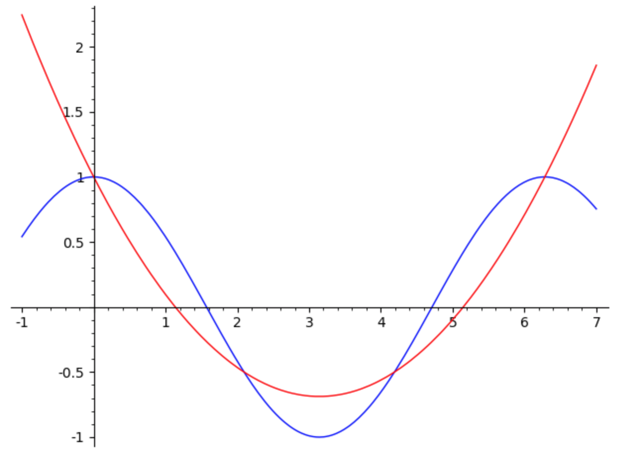
The following example obtained with the SageMath product illustrates the Lagrange interpolation for the function \(y=\cos(x)\), with \(n=3\), in the interval \([0,2\pi]\).
3.2) Hermite interpolation
The purpose of the Hermite interpolation is to improve the Lagrange approximation, imposing the further condition that also the derivatives have the same value at the control points.
Definition 3.1
Let \(f(x)\) be a function with continuous first derivative in the interval \([a,b]\), in symbols \( f \in C^{1}[a,b]\). Let \((x_{0},x_{1},\cdots,x_{n})\) be distinct points in the interval \([a,b]\). The Hermite interpolating polynomial \(p(x)\) has the following properties:
Theorem 3.4 – Hermite
Let \(f(x)\) be a function of class \(C^{1}[a,b]\) and \(x_{0},x_{1},\cdots,x_{n}\) be \(n+1\) distinct points in the interval. Then there exists a single interpolating polynomial of degree less than or equal to \(2n+1\), given by the following expression:
where \(H_{n,i}(x)\) and \(K_{n,i}(x)\) are polynomials connected to Lagrange polynomials \(L_{n,i}(x)\). The polynomial \(p(x)\) is called the first order osculating polynomial. We recall without proof the formulas for the polynomials \(H_{n,i}(x)\) and \(K_{n,i}(x)\):
\[ \begin{array}{l} H_{n,i}(x) =[1- 2(x-x_{i})L_{n,i}^{‘}(x_{i})](L_{n,i}(x))^{2} \\ K_{n,i}(x) = (x-x_{i})(L_{n,i}(x))^{2} \end{array} \]We note that in the case of a single point \(x_{0}\) the osculating polynomial is reduced to the Taylor polynomial.
For a complete study of Lagrange and Hermite interpolation see [2] or [3].
4) Bernstein polynomials
The set consisting of all polynomials with real coefficients of degree less than or equal to \(n\) has a vector space structure; the polynomials can be added together and multiplied by a scalar quantity.
A natural basis for this vector space is the set of polynomials \(\{1,x,x^{2},\cdots, x^{n}\}\). Any other polynomial of degree \(\le n\) can be expressed as a linear combination of these base polynomials. However, there are other possible bases; one of these is constituted by the Bernstein polynomials which we will now introduce.
Definition 4.1
Bernstein polynomials of degree \(n\) are defined as follows:
There are \(n+1\) Bernstein polynomials of degree \(n\). Bernstein polynomials of degree \(n\) form a base for the set of polynomials.
Bernstein polynomials of degree 1 are:
Bernstein polynomials of degree 2 are:
\[ \begin{array}{l} B_{2,0}(t) = (1-t)^{2} \\ B_{2,1}(t) = 2t(1-t) \\ B_{2,2}(t) = t^{2} \\ \end{array} \]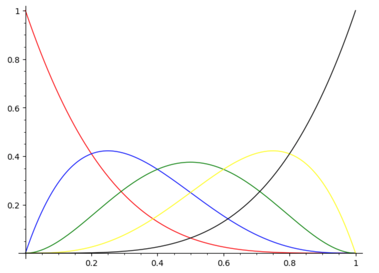
From the definition, the following properties easily follow:
Theorem 4.1
\[ \begin{array}{l} B_{n,k}(t) \ge 0 \quad \text{$ \forall t\in [0,1]$} \\ B_{n,k}(t) =B_{n,n-k}(1-t) \\ B_{n,k}(t)= (1-t)B_{n-1,k}(t) +tB_{n-1,k-1}(t)\\ \end{array} \]Exercise 4.1
Prove the following formulas:
Bernstein’s polynomials can be used to prove the following famous and important Weierstrass (1815-1897) theorem:
Theorem 4.2 – Weierstrass
Let us define a continuous function in the interval \([0,1]\). Then for every fixed \(\epsilon \gt 0\) there exists a polynomial \(p(x): [0,1] \to \mathbb{R}\) such that
We can formulate the theorem in an equivalent form. We define the Bernstein polynomial function:
\[ f_{n}(x) = \sum_{k=0}^{n} f\left(\frac{k}{n}\right) B_{n,k}(x) \]Then the sequence of polynomials \(f_{n}(x)\) converges uniformly to the function \(f(x)\) in its domain of definition \([0,1]\). For an in-depth analysis of Bernstein’s polynomials and the proof of Weierstrass’s theorem see for example [4].
5) Splines
In many applications the objects to be represented cannot be precisely defined by simple curves, such as arcs, ellipses, etc. Modeling curves (or even surfaces) are often created from a set of representative points of the object. The points and directions of the tangents at each point are used to determine the equation of the polynomial that approximates the shape of the curve. The resulting curve passing through the points is called an interpolating spline.
Other types of splines do not pass through all points; some are used to control and model the shape of the curve in the vicinity of each point. The resulting curve is called the approximating spline.
The most used splines are those of the third degree.
5.1) Cubic spline
Let \(n+1\) points or nodes \({x_{0},x_{1}, \cdots, x_{n}}\) be given, with \(x_{0} \lt x_{1} \lt \cdots \lt x_{n}\). A cubic spline of degree 3 is a composite function \(S_{3,n}(x)\) defined in the interval containing the points:
\[ S_{3,n}(x)= \begin{cases} p_{1}(x) \quad x \in [x_{0},x_{1}] \\ p_{2}(x) \quad x \in [x_{1},x_{2}] \\ \vdots \\ p_{n}(x) \quad x \in [x_{n-1},x_{n}] \\ \end{cases} \]The function \(S_{3,n}(x)\) is a collection consisting of \(n\) polynomials \(p_{i}(x)\) of degree \(3\) at most.
Now suppose we have, for each point \(x_{i}\), a value \(f(x_{i})\). The spline \(S_{3,n}(x)\) is called an interpolating cubic spline with respect to the data pairs \((x_{i},f_{i})\) if it results:
Clearly, inside each interval \([x_{i-1},x_{i}]\) the polynomial \(p_{i}(x)\) has derivatives of all orders. The discontinuity points of the spline \(S_{3,n}(x)\) can only be in the nodes. In general, additional continuity conditions are imposed in the nodes:
\[ \begin{array}{l} p_{i-1}(x_{i})=p_{i}(x_{i}) \\ p_{i}'(x_{i}) = p_{i+1}'(x_{i}) \\ p_{i}”(x_{i}) = p_{i+1}”(x_{i}) \\ \end{array} \]Different types of spline curves can be defined by setting different boundary conditions in the nodes. For a systematic study of the various types of splines (natural, complete and others) and their properties see Quarteroni’s bibliography.
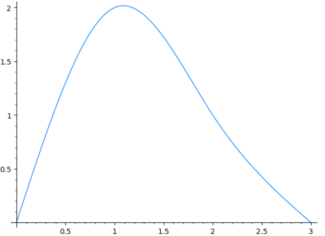
Exercise 5.1
Determine the natural first order spline to approximate the following data: \((0,0),(1,2),(2,1),(3,0)\).
Solution
The curve obtained with the SageMath tool is the following:
5.2) Cubic spline of Hermite
A cubic Hermite spline tries to control the shape of the curve by imposing conditions on the tangents at the extreme points.
Definition 5.2
Let \([a,b]\) be an interval and \(f: [a,b] \to\mathbf{R}\) a derivable function. Let \((x_{0}, \cdots, x_{n})\) be a partition. Hermite’s cubic spline is a finite set of polynomials \(p_{0}, \cdots,p_{n-1}\) satisfying the following relations:
for \(i=0,1, \cdots, n-1\).
Each component of the Hermite cubic spline has the following representation:
where \(p_{0},p_{1}\) are the starting and ending points, \(v_{0},v_{1}\) are the tangents at the points, and the polynomials \(H_{i}(t)\) have the following expression
\[ \begin{split} H_{0}(t)&= (1+2t)(1-t)^{2} \\ H_{1}(t)&= t(1-t)^{2} \\ H_{2}(t)&= t^{2}(t-1) \\ H_{3}(t)&= t^{2}(3-2t) \\ \end{split} \]We can give this matrix representation:
\[ p(t)= \left( \begin{array}{cccc} p_{0} &v_{0}& v_{1} & p_{1} \end{array} \right) \cdot \left( \begin{array}{cccc} 1 &0 & -3 &2 \\ 0 & 1 & -2 &1 \\ 0 &0 & -1 & 1 \\ 0 &0 & 3 & -2 \end{array} \right) \cdot \left( \begin{array}{c} 1 \\ t \\ t^{2} \\ t^{3} \end{array} \right) \\ \]or the following equivalent one:
\[ p(t) = \left( \begin{array}{cccc} t^{3} &t^{2} & t & 1 \end{array} \right) \cdot \left( \begin{array}{cccc} 2 & -2 & 1& 1 \\ -3 & 3 & -2 & -1 \\ 0 & 0 & 1 & 0 \\ 1 & 0 & 0 & 0 \end{array} \right) \cdot \left( \begin{array}{c} p_{0} \\ p_{1} \\ v_{0} \\ v_{1} \end{array} \right) \\ \]Unlike Bézier curves, the Hermite shape of a curve is not a weighted average, as the sum \(H_{0}+H_{1}+H_{2}+H_{3}\) is generally not equal to \(1\). The coefficients \(H_{0},H_{3}\) are the starting and ending points, while the coefficients \(H_{1},H_{2}\) are vectors.
5.3) The Catmull-Rom splines
The Hermite spline is simple to compute and allows you to create a smooth and symmetrical compound curve. To modify the curve, you can modify the position of a node or the direction of the tangent in the node. However it has the disadvantage of needing to know the derivatives at the nodes.
If the derivatives are not known, they can be approximated with finite differences. This is the approach proposed by E. Catmull and R. Rom in 1974 [5].
One of the characteristics of the Catmull-Rom spline is that the curve passes through all control points, unlike other types of splines.
As we know, the spline is a collection of cubic curves connected to each other at the extreme points. The first curve goes from point \(p_{0}\) to point \(p_{1}\), the second from point \(p_{1}\) to point \(p_{2}\), etc. To have continuity in the connecting points of the curves, the two tangents must be equal. The standard Catmull-Rom splines procedure creates the tangent at a point using neighboring points. The formula for the tangent \(\mathbf{v}_{i}\) at point \(p_{i}\) is
The important fact is that to calculate the tangent at a point it is enough to know the position of the adjacent points.
The procedure for determining the Catmull-Rom spline is similar to that used for the Hermite spline; the matrix representation is:
6) The Bézier curves
Bézier curves represent a fundamental class of spline curves. The name derives from Pierre Bézier (1920-1999), who first published an article while working at the Renault car manufacturer as engineer and designer. Actually the same type of curves had already been studied by Paul de Casteljau while working at Citroën, but he did not publish his research.
Definition 6.1
Let \(n+1\) points \({p_{0},p_{1}, \cdots , p_{n}}\) be given. The Bézier curve is defined by the following equation
where \(B_{n,k}(t)\) are the Bernstein polynomials. The main properties of the Bézier curve are the following:
- the curve passes through the starting and ending points \(p_{0}\) e \(p_{1}\);
- the curve lies in the convex region delimited by the points, as \(B_{n,k}(t) \ge 0\), for each \(t \in [0,1]\);
- the curve is tangent at the extreme points to \(p_{1}-p_{0}\) and \(p_{n}-p_{n-1}\).
These points are called control points. The broken line formed by the segments that join them is called the control polygon . Only the first and last control points belong to the Bézier curve, while the rest control the shape of the curve in their proximity. It is therefore an approximating curve and not an interpolating curve.
The Bernstein polynomials serve as blending functions for the Bézier curves, that is, as weights associated with the control points. The order of the polynomial representing the curve is equal to the number of control points minus one.
A disadvantage of the Bézier curves is the lack of local control over the curve. If we modify a control point the whole curve is modified, not just the local part near the point.
6.1) Cubic Bézier curves
The most commonly used Bézier curves are those of the third degree, defined by four control points. In this case the Bernstein polynomials are as follows:
\[ \begin{array}{l} B_{3,0}(t) =(1-t)^{3} \\ B_{3,1}(t) =3t(1-t)^{2} \\ B_{3,2}(t) =3t^{2}(1-t) \\ B_{3,3}(t) =t^{3} \\ \end{array} \]Exercise 6.1
Prove the following relations satisfied by the first derivative of the cubic Bézier curve:
6.2) Matrix representation of the Bézier cubics
The cubic Bézier curve (case \(n=3\)), with \(4\) control points \({p_{0},p_{1},p_{2},p_{3}}\), has the following vector expression:
\[ p(t) = (1-t)^{3}p_{0}+3t(1-t)^{2}p_{1}+3t^{2}(1-t)p_{2}+t^{3}p_{3} \]In matrix form it can be written as follows:
\[ p(u) = \left( \begin{array}{cccc} t^{3} &t^{2} & t & 1 \end{array} \right) \cdot \frac{1}{2} \cdot \left( \begin{array}{cccc} -1 & 3 & -3 & 1 \\ 3 & -6 & 3 & 0 \\ -3 & 3 & 0 & 0 \\ 1 & 0 & 0 & 0 \end{array} \right) \cdot \left( \begin{array}{c} p_{0} \\ p_{1} \\ p_{2} \\ p_{3} \end{array} \right) \\ \]Exercise 6.2
Draw the Bézier curve for the following \(4\) points:
Solution
The curve in the plane is represented by the following pair of parametric equations:
The Bézier spline plot is as follows:
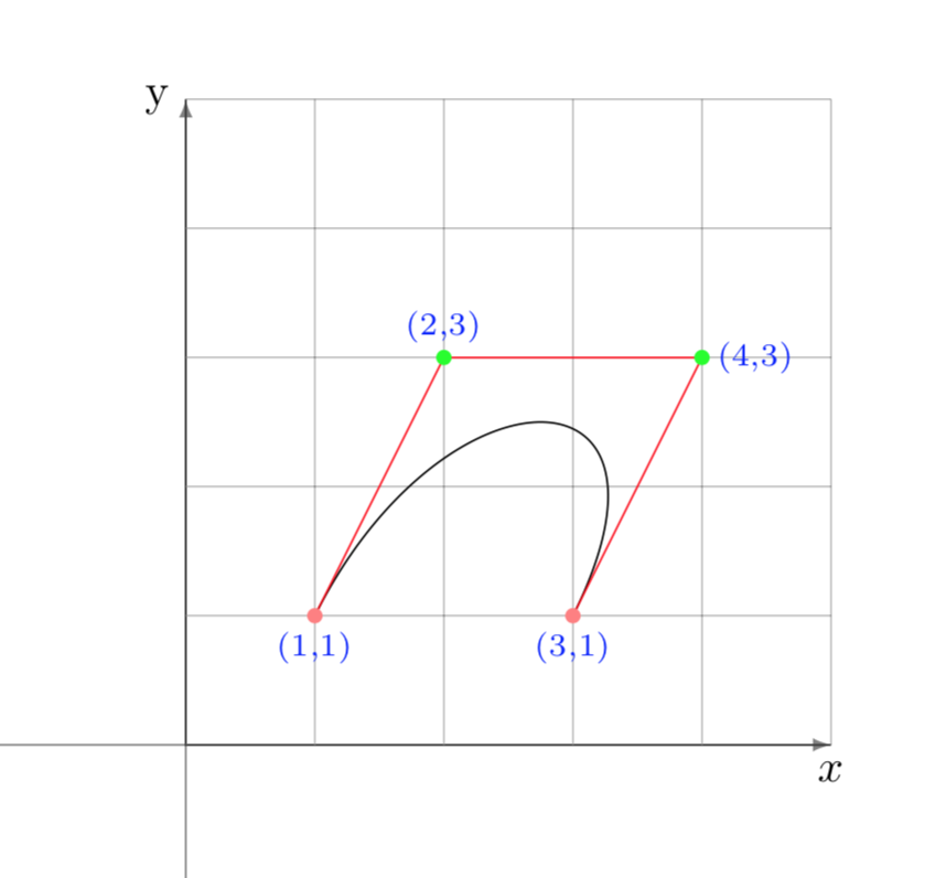
The graph was created with the TikZ product in the Latex environment, using the following instruction:
<pre class="wp-block-code"><code>\draw[scale=1,domain=0:1,samples=100,variable=\t]
 plot ({(1-\t)^3 +6*\t*(1-\t)^2 +12*\t^2*(1-\t)+3*\t^3},
       {(1-\t)^3 +9*\t*(1-\t)^2 +9*\t^2*(1-\t)+\t^3});</code></pre>
This way of calculating the Bézier curve is good if you have few nodes. As the number of nodes increases, the degree of the polynomial increases and numerical instabilities and rounding errors occur.
A better way is to use de Casteljau’s algorithm.
6.3) The de Casteljau algorithm
In \(1959\) Paul de Casteljau (1910-1999) created a simple and efficient algorithm that constructs a Bézier curve through repeated linear interpolations.
The algorithm starts by setting a value of the parameter \(t \in(0,1)\). Between each pair of consecutive control points a linear interpolation is made according to the parameter \(t\), obtaining a new point. Starting from the initial \(4\) control points denoted with the notation \((p_{0}^{0},p_{1}^{0},p_{2}^{0},p_{3}^{0})\), we get \(3\) new points \((p_{0}^{1},p_{1}^{1},p_{2}^{1})\). We continue until we obtain a single point \(p_{0}^{3}\), which is the desired value of the polynomial in \(t\): \(p(t)\). In each step of the algorithm, a new point is created between each pair in the ratio \(t:(1-t)\).
We can summarize the algorithm with these recurrence equations:
To see de Casteljau’s algorithm in action see this link to Wikipedia.
7) Use of Bézier curves in video games
Splines are used in various situations in video game programming:
- to control the movement of an NPC (Non-Player Character) character, so that its motion is as fluid and realistic as possible. This is guaranteed by the continuity of the first and second derivatives of the spline;
- to describe different paths;
- to model objects of various geometric shapes;
- in Unity animations, to define useful curves in keyframe interpolation (see article on this website).
7.1) Generation of a Catmull-Rom spline
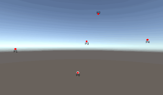
The Catmull-Rom spline is useful for calculating a curve that passes through all control points. For example, it can be used to calculate the curve of an object from keyframes in an animation process.
The following animation illustrates an object that moves through \(5\) fixed points, following a curved trajectory created with the Catmull-Rom algorithm.
The instructions for calculating the points of the curve are the following:
//compute position on Catmull-Rom spline, relative to t
Vector3 ComputePositionCatmullRom(float t, Vector3 p0,  Vector3 p1, Vector3 p2, Vector3 p3) {
    Vector3 position = 0.5f * (2*p1 + (p2-p0)*t +
              (2*p0-5*p1+4*p2-p3)*t*t +
              (-p0+3*p1-3*p2+p3)*t*t*t);

    return position;
}
7.2) Motion along a Bézier curve
In some situations, Bézier curves are used to define a path through which an object must move.
The following animation refers to a butterfly-shaped path, consisting of \(4\) paths connected at the junction points.
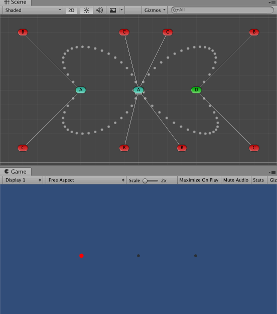
Each path is created using a distinct Bézier curve, with \(4\) control points. The fourth control point of each curve coincides with the first of the next. The Update function activates a coroutine to calculate the individual routes, using the Bézier formula:
private IEnumerator MotionOnPath(int  number) {

    // p0,p1,p2,p3  are control points
    ..............
    while (t < 1) {
        t += Time.deltaTime * velocityFactor;
        pointComputed =
             Mathf.Pow(1 - t, 3) * p0 +
             3 * Mathf.Pow(1 - t, 2) * t * p1 +
             3 * (1 - t) * Mathf.Pow(t, 2) * p2 +
             Mathf.Pow(t, 3) * p3;
        transform.position = pointComputed;
        yield return new WaitForEndOfFrame();
    }
    ..............
}
By modifying the number of component curves and changing the positions of the control points, it is possible to create an infinite number of different curves which can be adapted to various situations.
7.3) Constant speed along a Bézier curve
The graph of a curve \(p(t)=(x(t),y(t))\) can be thought of as the trajectory of a particle moving in the plane, with \(p(t)\) indicating the position at the time \(t\). The velocity of the particle is given by the following vector equation:
\[ v(t) = \frac{dp}{dt} \]We denote the modulus of velocity as \(\sigma(t)\):
\[ \sigma (t) = |v(t)| \]Generally the modulus of speed is not constant, but it varies according to the parameter. A fundamental parameter is the curvilinear abscissa \(s(t)\), which indicates the distance traveled in the time \(t\). The curvilinear abscissa is defined as follows:
\[ s=g(t) = \int_{t_{0}}^{t}\left|\frac{dp}{dt}\right|dt \]where \(\left|\frac{dp}{dt}\right|= \sqrt{x'(t)^{2}+ y'(t)^{2}}\). If we use the parameter \(s\) we can see that the velocity module is constant and equal to \(1\).
Example 7.1 – The circumference
The circumference of a circle, with center \((0,0)\) and radius equal to \(1\), has the following parametric equations expressed with the curvilinear abscissa:
We can use a different parametrization, for example the following, in which the velocity is not constant:
\[ \begin{split} p(t) &=(\cos (t^{2}), \sin (t^{2})) \quad t \in [0,\sqrt{2\pi}] \\ v(s) &=(-2t\sin (t^{2}), 2t\cos (t^{2})) \\ \sigma (t) & = 2t \end{split} \]In various situations we need a constant velocity for an object along a curve (for example, in regard to the motion of a camera). If we have a curve of equation \(q(t)\) and we want the velocity to be constant, we must find the relation of the parameter \(t\) with the curvilinear abscissa \(t=f(s)\). This process is called reparametrization. Assuming that \(p(s)\) is a natural parametrization with the curvilinear abscissa, we must set \(p(s)=q(t)\) and solve with respect to \(t\). In the case of the above example of the circle the solution is easy: \(t=\sqrt{s}\). In the general case the following integral must be calculated, for each value of \(t\):
\[ s=g(t) = \int_{t_{0}}^{t}\left|\frac{dq}{dt}\right|dt \]This integral equation, fixed a value of \(t\), allows to calculate the length \(s(t)\). The calculation of this integral generally requires the use of numerical analysis methods, among which one of the simplest is the Cavalieri-Simpson method (Wikipedia).
In reality, the inverse function is needed; given a value of \(s\) determine the time \(t\) in which the length takes on that value: \(t = g^{-1}(s)\). Except in the simplest cases, generally there is no solution in closed form, but one must use the methods of numerical analysis.
The most famous algorithm is Newton’s method for finding the zeros of a function (Wikipedia). The function in question is \(F(t)=g(t)-s\) where \(s\) is a fixed constant value. Newton’s method for finding the zeros of \(F(t)\) is based on the following iteration:
where \(F'(t)=|\frac{dq}{dt}|\).
So, in summary, given a Bézier curve \(p(t)\), if we want the object (Game Object) to move along the curve at a constant speed, we must take the following steps:
- determine the total length of the curve, using Simpson method or another method for calculating the approximate integral;
- divide the curve into sections of equal length, and for each value of the parameter \(s\) determine the corresponding value of the parameter \(t\), using Newton’s method;
- calculate \(p(t)\) with the Bézier formula.
For Simpson’s method and Newton’s algorithm see a numerical analysis text, for example Quarteroni’s book.
Conclusion
Splines are of great importance in game development. Developers need to have an understanding of the properties of various types of curves and choose the best for the problem. For completeness, in a future article we will describe two other types of curves: B-Splines and NURBS.
Bibliography
[1]Seymour Lipschutz – Schaum’s Outline of Linear Algebra (McGraw-Hill)
[2]A. Quarteroni, R. Sacco – Numerical Mathematics (Springer Verlag)
[3]F. Scheid – Numerical Analysis (McGraw-Hill)
[4]G. Lorentz – Bernstein Polynomials (Ams Chelsea Publishing)
[5]E. Catmull, R. Rom – A Class of Local Interpolating Splines (from ‘Computer Aided Geometric Design’, by Academic Press, 1974)

0 Comments