Lambert Series, the Arithmetic Function r(n) and Gauss’s Probability Integral

In this article we will study some properties of Lambert series. Then, using Lambert series relative to the representation of integers as sum of two squares, we will compute the value of Gauss’s classical probability integral.

---

1) Dirichlet generating functions

Let’s briefly recall some properties of Dirichlet generating functions.

Definition 1.1
Given an arithmetic function \(f(n\)), the associated Dirichlet generating function is the following series:

\[ F(s)= \sum\limits_{n=1}^{\infty}\frac{f(n)}{n^{s}} \]

where \(s=\sigma + it\) is a complex number.

Regarding the problem of convergence, recall that for each Dirichlet series there is a real number \(\sigma_{0}\), called abscissa of absolute convergence, such that the series converges absolutely in the half-plane \(\sigma \gt \sigma_{0}\), to the right of \(\sigma_{0}\).
It can be shown that in the region of absolute convergence the Dirichlet series represents the arithmetic function \(f(n)\) uniquely; that is, if two arithmetic functions are different their corresponding Dirichlet series are also different.

Example 1.1
The most famous and important Dirichlet series is the Riemann zeta function:

\[ \zeta(s)=\sum\limits_{n=1}^{\infty}\frac{1}{n^{s}} \]

The abscissa of absolute convergence of \(\zeta(s)\) is equal to \(1\).

The inverse of the zeta function has the following Dirichlet generating function:

\[ \frac{1}{\zeta(s)}=\sum\limits_{n=1}^{\infty}\frac{\mu(n)}{n^{s}} \]

where \(\mu(n)\) is the function of Mobius. Recall that the Möbius function \(\mu(n)\) is defined as follows:

\[ \mu(n)= \begin{cases} 1 \quad \quad \quad \text{if } n=1 \\ (-1)^{k} \quad \text{if } n=\prod\limits_{i=1}^{k} p_{i} \\ 0 \quad \quad \quad \text{if } n \quad \text{has a prime square factor} \end{cases} \]

For the Möbius function see the article in this blog.

Example 1.2
We define the following arithmetic function (also called Dirichlet character):

\[ \chi (n)= \begin{cases} 0 \quad \quad \quad \quad 2|n \\ (-1)^{\frac{n-1}{2}} \quad 2 \nmid n \end{cases} \]

The Dirichlet character therefore assumes the value \(+1\) for all odd numbers of the form \(4k+1\), and the value \(-1\) for all odd numbers of the form \(4k+3\).

The associated Dirichlet series is:

\[ L(s)=\sum\limits_{n=1}^{\infty}\frac{\chi(n)}{n^{s}}= 1^{-s}-3^{-s}+5^{-s}- \cdots \]

Exercise 1.1
Prove that the function \(\chi(n)\) is completely multiplicative. That is, for every pair of positive integers \(n,m\) we have:

\[ \chi(nm)=\chi(n)\chi(m) \]

Definition 1.2
Given two arithmetic functions \(f(n),g(n)\), we define the product (or convolution) of Dirichlet the following arithmetic function:

\[ h(n)=(f*g)(n)=\sum\limits_{d|n}f(d)g\left(\frac{n}{d}\right) \]

The following theorem holds:

Theorem 1.1
Let two arithmetic functions \(f(n),g(n)\) be given, with respective Dirichlet generating functions \(F(s),G(s)\). Then, in the half-plane in which both series converge absolutely, the generating function \(H(s)\) of the convolution \(f*g\) is the following:

\[ H(s)=\sum\limits_{n=1}^{\infty}\frac{(f*g)(n)}{n^{s}}= F(s)G(s) \]

Proof
We write the product of the two series:

\[ F(s)G(s)= \sum\limits_{n=1}^{\infty}\frac{f(n)}{n^{s}} \sum\limits_{n=1}^{\infty}\frac{g(n)}{n^{s}}= \sum\limits_{n=1}^{\infty} \sum\limits_{m=1}^{\infty} \frac{f(n)g(n)}{(nm)^{s}} \]

Thanks to absolute convergence we can multiply and reorder the two series as we want, without changing the result. To conclude the proof, we simply group the terms with the constant product \(nm=k\) and write the series relative to the product.

From the previous theorem the following theorem easily derives:

Theorem 1.2
Suppose that

\[ g(n)=\sum\limits_{d|n}f(d) \]

and \(F(s),G(s)\) are the Dirichlet generating functions of \(f(n),g(n)\). Then

\[ \begin{array}{l} f(n) = \sum\limits_{d|n}g(d)\mu \left(\dfrac{n}{d}\right) \\ G(s) = \zeta(s) F(s) \end{array} \]

For an in-depth study of the Dirichlet series consult a book about number theory, for example ^[1] or ^[3] .

Theorem 1.3

\[ \begin{array}{l} \zeta^{2}(s) = \sum\limits_{n=1}^{\infty}\dfrac{d(n)}{n^{s}} \\ \end{array} \]

where \(d(n)\) is the arithmetic function that counts the number of divisors of \(n\) (see the article in this blog).

Hint
Use theorem 1.2.

---

2) The generating functions of Lambert

Despite the importance of Dirichlet functions, there are other possible generating functions. Among these are the Lambert series (1728-1777), which have the following form:

\[ \sum\limits_{n=1}^{\infty}a_{n}\frac{x^{n}}{1-x^{n}} \]

If the series \(\sum\limits_{1}^{\infty}a_{n}\) converges, then the Lambert series converges for all values ​​of \(x\), except for \(x \pm 1\). Otherwise it converges for the values ​​of \(x\) for which the power series \(\sum\limits_{n=1}^{\infty}a_{n}x^{n}\) converges. 
In the case \(a_{n}=1\), if \( |x| \lt 1\) the fraction \(\dfrac{x^{n}}{1-x^{n}}\) is the sum of a geometric series and thanks to absolute convergence the series can be reordered without changing the sum.

Theorem 2.1
If the Lambert series converges absolutely we have:

\[ \sum\limits_{n=1}^{\infty}a_{n} \frac{x^{n}}{1-x^{n}}= \sum\limits_{n=1}^{\infty} b_{n}x^{n} \]

where

\[ b_{n}= \sum\limits_{d|n} a_{d} \]

Proof
The absolute convergence allows to reorder the terms of the series, grouping all the terms that give a constant value \(mn=k\), relative to the power \(x^{k}\). For example, to compute the coefficient of  \(x^{6}\), we can add the coefficients with all the divisors of \(6\): \(a_{1},a_{2},a_{3},a_{6}\). So we have

\[ \sum\limits_{n=1}^{\infty}a_{n}\frac{x^{n}}{1-x^{n}}= \sum\limits_{n=1}^{\infty} a_{n}\sum\limits_{m=1}^{\infty} x^{mn}= \sum\limits_{n=1}^{\infty} b_{n}x^{n} \]

where

\[ b_{n}= \sum\limits_{d|n} a_{d} \]

The following theorem holds:

Theorem 2.2
Suppose that \(A(s),B(s)\) are the Dirichlet series relative to the coefficients \(a_{n},b_{n}\). Then:

\[ \sum\limits_{n=1}^{\infty}a_{n} \frac{x^{n}}{1-x^{n}}= \sum\limits_{n=1}^{\infty} b_{n}x^{n} \]

if and only if

\[ \zeta(s)A(s)=B(s) \]

Exercise 2.1

\[ \sum\limits_{n=1}^{\infty}\mu(n) \frac{x^{n}}{1-x^{n}}= x \\ \]

Exercise 2.2

\[ \sum\limits_{n=1}^{\infty}d(n)x^{n} = \frac{x}{1-x}+\frac{x^{2}}{1-x^{2}}+\frac{x^{3}}{1-x^{3}}+ \cdots \\ \]

Hint
Use theorem 1.3 and theorem 2.1.

Exercise 2.3
Prove that if

\[ \begin{array}{l} F(x) = \sum\limits_{n=1}^{\infty}a_{n}\dfrac{x^{n}}{1-x^{n}} \quad and \quad G(x) = \sum\limits_{n=1}^{\infty} a_{n}x^{n} \\ \end{array} \]

then

\[ \begin{array}{l} F(x) = \sum\limits_{n=1}^{\infty}G(x^{n}) \\ \end{array} \]

---

3) The arithmetic function \(r(n)\)

We define the arithmetic function \(r(n)\) as the number of representations of \(n\) in the form

\[ n=x^{2}+y^{2} \quad x,y \in \mathbb{Z} \]

The representations that differ in signs or order are counted as distinct. For example \(r(5)=8\) because

\[ 5=(\pm 1^{2})+(\pm 2^{2})=(\pm 2^{2})+(\pm 1^{2}) \]

For number \(4\) we have

\[ 4=(\pm 0^{2})+(\pm 2^{2})=(\pm 2^{2})+(\pm 0^{2}) \]

In the case of a composite number, the conditions for representing an integer as the sum of two squares are contained in the following Fermat theorem:

Theorem 3.1 – Fermat
Let a positive integer \(n\) with the following prime factorization:

\[ n = 2^{t}\prod_{i}p_{i}^{r_{i}} \prod_{j}q_{j}^{s_{j}} \]

where  \(p_{i} \equiv 1 \pmod{4}\) and \(q_{j} \equiv 3 \pmod{4}\). Then it is possible to write  \(n=x^{2}+ y^{2}\) if and only if all the exponents \(s_{j}\) are even.

For a proof see one of the texts in the bibliography.

The following theorem has been proved by Jacobi through his theory of elliptic functions. However, an equivalent form had also been proved by Gauss in his fundamental work ‘Disquisitiones Arithmeticae’, published in 1801 in Latin.

Theorem 3.2 – Jacobi-Gauss

\[ r(n)=4(d_{1}(n) – d_{3}(n)) \]

where \(d_{1}(n),d_{3}(n)\) are the number of divisors of the form \(4n+1\) and \(4n+3\) respectively. For a proof see ^[2].

Example 3.1
In the case \(n=10\) we have \(r(10)=8\). The divisors of type \(4k+1\) are \(1,5\). There are no divisors of type \(4k+3\). Then

\[ r(10)= 4(d_{1}(10) – d_{3}(10))=4 \cdot 2=8 \]

We note that, from the definition of the Dirichlet character, it results:

\[ d_{1}(n)-d_{3}(n)=\sum\limits_{d|n}\chi(d) \]

---

4) The generating function of \(r(n)\)

We can now go back to our function \(r(n)\). Based on theorem 3.2 we can write

\[ r(n)=4 \sum\limits_{d|n}\chi(d) \]

For theorem 1.2 we have then

\[ \sum\limits_{n=1}^{\infty}\frac{r(n)}{n^{s}}=4\zeta(s)\sum\limits_{n=1}^{\infty}\frac{\chi(n)}{n^{s}} \]

From the previous relation and from theorem 2.1 we easily prove the following theorem:

Theorem 4.1

\[ \sum\limits_{n=1}^{\infty}r(n)x^{n} = 4 \left(\frac{x}{1-x}-\frac{x^{3}}{1-x^{3}}+\frac{x^{5}}{1-x^{5}}- \cdots \right) \\ \]

Now consider the following series

\[ S= 1+2x+2x^{4}+2x^{9}+\cdots \]

If we calculate the square \(S^{2}\) of the series, we obtain a series of powers in which the coefficient in front of \(x^{n}\) is precisely \(r(n)\). In fact, every pair of exponents \( i,k\) such that \(i^{2}+k^{2}=n\) contributes to the coefficient with a unit value. From this observation we can write the previous theorem in this equivalent form:

Theorem 4.2

\[ (1+2x+2x^{4}+2x^{9}+\cdots)^{2}=1+4\left(\frac{x}{1-x}-\frac{x^{3}}{1-x^{3}}+\frac{x^{5}}{1-x^{5}}- \cdots \right) \]

In the following paragraphs we will use this formula to calculate Gauss’s integral.

---

5) Gauss’s probability integral

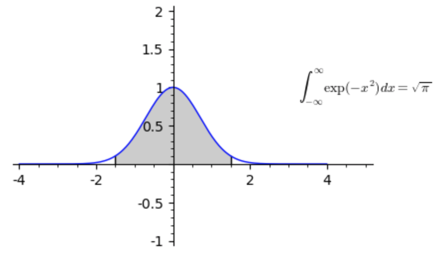
The Gaussian integral is the integral of the function \(f(x)=e^{-x^{2}}\) calculated on the whole real axis:

\[ \begin{array}{l} \int\limits_{- \infty}^{\infty}e^{-x^{2}} dx = \sqrt{\pi} \end{array} \]

The function \(e^{-x^{2}}\) is symmetric with respect to the origin, therefore it is sufficient to calculate the integral only on the positive real half-line:

\[ I= \int\limits_{0}^{\infty}e^{-x^{2}} dx = \frac{\sqrt{\pi}}{2} \\ \]

Even if it is connected to the name of Gauss, the integral was already known to De Moivre (1667-1754) in his studies on the calculus of probability, in particular in his book ‘The Doctrine of Chances’ of 1718. It was also subject of study by Laplace (1749-1827).

The Gaussian integral cannot be calculated with elementary methods. One of the simplest methods is probably that of Poisson (1781-1840), which consists in calculating the double integral

\[ \int\limits_{-\infty}^{\infty} \int\limits_{-\infty}^{\infty} e^{-(x^{2}+y^{2})}dx dy \]

using polar coordinates, and take advantage of the fact that the double integral can be expressed as the product of the two partial integrals. For details see a text of mathematical analysis.
Assuming we know the value of the Gaussian integral, we can prove the following theorem:

Theorem 5.1

\[ \alpha = \lim_{x \to 1-0}\sqrt{1-x}(1+x +x^{4}+x^{9}+ \cdots + x^{n^{2}}+ \cdots)=\frac{\sqrt{\pi}}{2} \]

Hint
Use the formula for the approximation of the integral of the function \(f(x)=e^{-x^{2}}\) through the Riemann sums:

\[ \int\limits_{\delta}^{\infty}f(x)dx\le \delta \sum\limits_{n=1}^{\infty}f(\delta n) \le \int\limits_{0}^{\infty}f(x)dx \]

Knowing the value of the Gaussian integral, we can easily deduce that \(\alpha= I=\dfrac{\sqrt{\pi}}{2}\).

---

6) Calculation of Gauss’s probability integral using Lambert series

Suppose now that we do not know the value of the Gaussian integral. If we are able to calculate the limit of the previous theorem in an alternative way, we could calculate the Gaussian integral. Based on theorem 4.2 we can write:

\[ \begin{array}{l} \alpha ^{2}= \lim\limits_{x \to 1-0} \left(1-x \right) \left(1+x +x^{4}+x^{9}+ \cdots + x^{n^{2}}+ \cdots \right)^{2} \\ = \dfrac{1}{4}\lim\limits_{x \to 1-0} \left(1-x\right)\left(2+ 2x +2x^{4}+2x^{9}+ \cdots + 2x^{n^{2}}+ \cdots\right)^{2} \\ = \dfrac{1}{4} \lim\limits_{x \to 1-0}\left(1-x \right) \left(1+4\left(\dfrac{x}{1-x}-\dfrac{x^{3}}{1-x^{3}}+\dfrac{x^{5}}{1-x^{5}}- \cdots \right)\right) \\ = \lim\limits_{x \to 1-0}\left(1-x \right) \left(\dfrac{x}{1-x}-\dfrac{x^{3}}{1-x^{3}}+\dfrac{x^{5}}{1-x^{5}}- \cdots \right) \\ \end{array} \]

The transition from the second to the third expression is easily justifiable. Let us now remember the famous formula of Leibniz (1646-1716):

\[ 1 -\frac{1}{3}+\frac{1}{5}- \frac{1}{7}+ \cdots = \frac{\pi}{4} \]

Using the Leibniz formula we can complete the calculation of the limit, obtaining the following result:

\[ \alpha ^{2}= 1 -\frac{1}{3}+\frac{1}{5}- \frac{1}{7}+ \cdots = \frac{\pi}{4} \]

So we can conclude that the value of the Gaussian integral is

\[ I = \alpha = \frac{\sqrt{\pi}}{2} \]

---

Conclusion

We have seen in this article an example of how a result that strictly belongs to the Theory of Numbers can be used to prove theorems and properties of Mathematical Analysis. This confirms once again the profound unity of Mathematics. In the next articles we will study other properties of the Dirichlet series and the Lambert series.

---

Bibliography

^[1]Niven, Zuckerman, Montgomery – An introduction to the Theory of Numbers (V edition, Wiley, 1991)

^[2]W. LeVeque – Fundamentals of Number Theory (Dover)

^[3]Hardy, Wright – An Introduction to the Theory of Numbers (Oxford University Press)