In a previous article we have introduced some examples of fractals, illustrating their main characteristics, both qualitative and quantitative: self-similarity, geometric irregularity, fractional dimension. To continue the study of fractal science, it’s first necessary to give a more rigorous definition of the mathematical context in which fractal objects are defined.
Each fractal is a geometric shape that we can consider immersed in an Euclidean space \(\mathbb {R}^{n}\) of size \(n = 1,2,3\) or even larger. To define the mathematical space of fractals it’s necessary to recall some concepts on the topology of metric spaces.
1) Metric spaces
Definition 1.1
A metric space \((X, d) \) is a pair formed by a set \(X \) and a function \(d: X \times X \to \mathbb {R} \), called distance function, which satisfies the following axioms:
Example 1.1 – The discrete metric
Given a set \(X \), we define the following metric:
It’s easy to verify that the defined function, called discrete metric, satisfies the axioms and therefore the pair \((X, d) \) is a metric space.
Example 1.2 – The Euclidean metric
Let \(X = \mathbb {R ^ {n}} \) be the Euclidean space with \(n \) dimensions. If \(x, y \) are two points in space, with coordinates \((x_{i})\) and \((y_{i})\), the Euclidean metric is defined as follows:
Example 1.3 – The rational and irrational numbers
We have seen that the set of real numbers \(\mathbb {R} \) is a metric space with the metric \(d (x, y) = | x-y | \). As is known, real numbers are made up of rational numbers and irrational numbers; therefore \(\mathbb {R} = \mathbb{Q} \cup \mathbb{I} \), where \(\mathbb {Q} \) is the set of rational numbers and \(\mathbb {I} \) is the set of irrational numbers. These two subsets are metric spaces with Euclidean metric.
Example 1.4 – The Manhattan metric
In the plane \(\mathbb{R^{2}} \) in addition to the Euclidean metric we can define the following metric, called the Manhattan metric, or Taxicab metric. Living in a city where the streets have a grid configuration, north-south and east-west, to go from a point \(A \) to a point \(B \) by taxi, you cannot take the shortest road according to the Euclidean metric, but you must travel only horizontally and vertically. In this situation, given two points \(A(x_ {1}, y_ {1}) \) and \(B (x_{2}, y_{2}) \) of the plane, the minimum distance to travel from the point \(A \) to the point \(B \) is given by the following value:
To prove that the function defined above satisfies the axioms of metric spaces, remember that given any two real numbers \(x, y \) the following relation holds: \(| x + y | \le | x | + | y | \).
2) Topological spaces
Definition 2.1
A topological space is a pair \((X, A) \) consisting of a set \(X \) and a family of subsets of \(X \), denoted by \(A \), called the open sets, which satisfies the following axioms:
- A1 – the universe set \(X \) and the empty set \(\emptyset \) are open
- A2 – the union of any finite or infinite number of open sets is an open set
- A3 – the intersection of a finite number of open sets is an open set
The complement of an open set is called a closed set. The definition of topological space does not presuppose any algebraic structure on the set \(X \). To define a topological space, therefore, we only have to define which subsets are open.
Example 2.1 – The trivial or indiscrete topology
Let \(X \) be any set. The trivial (or indiscrete) topology on \(X \) is the topology in which \(A = \{\emptyset, X \} \), that is the open sets are only the trivial subsets.
Example 2.2 – The discrete topology
Let \(X \) be any set. Discrete topology defines all subsets of \(X \) as open. The family of all subsets of \(X \) is called the power set of \(X \), denoted by \(P (X) \).
Exercise 2.1
Prove that, if \(| X | = n \), then the number of open sets in the discrete topology is \(2^{n} \).
3) Topology in metric spaces
On every metric space \((X, d) \) we can define a topology induced by the metric.
Definition 3.1
Given a metric space \((X, d) \), we define the open sphere (or open ball) of radius \(r \) and center \(x \), the set
We now define open all subsets of \(𝑋\) which are union of open spheres. It’s easily proved that, with this definition of open sets, the set \(𝑋\) assumes a topological space structure.
Example 3.1
The Euclidean topology of \(\mathbb{R}^{n}\) is that induced by the Euclidean metric:
Definition 3.2 – Limit of a sequence
A sequence of points \(\{x_{n}\}\) of a metric space \((𝑋, 𝑑)\) converges to a point \(x \in X\) (or equivalently has limit at a point \(x \in X\)) as \(x\) goes to infinity, if the following condition holds:
In this case we use the following notation:
\[ \lim_{n \to \infty} {x_{n}} = x \]Definition 3.3 – Cauchy sequence
A sequence of points \(\{x_{n} \} \) of a metric space \((X, d) \) is called Cauchy sequence if the terms of the sequence eventually become arbitrarily close to one another; that is
Exercise 3.1
Prove that every convergent sequence is also a Cauchy sequence.
Definition 3.4 – Complete metric space
A metric space \((X,d)\) is said to be complete if each Cauchy sequence \(\{x_{n} \} \) is convergent to a point in \(X \).
Example 3.2
The open interval \(X = (0,1) \) of the real line is a metric space but it’s not complete. For example, the sequence \(\{x_ {n} = \frac {1}{n} \} \) is a Cauchy sequence but doesn’t converge to a point in the interval.
However, the closed interval \([0,1] \) is a complete metric space.
Definition 3.5 – Compact set
Let a metric space \((X, d) \) be given. A subset \(C \) of \(X \) is said to be compact if each infinite sequence \(\{x_{n} \} \) contains a subsequence that has limit belonging to \(C \).
The following fundamental theorem of mathematical analysis holds:
Theorem 3.1 – Heine-Borel
A subset of the Euclidean space \(R^{n} \) is compact if and only if it is closed and bounded.
For a deeper study of Topology and Metric Spaces you can consult [1]. Like all the texts in the Schaum’s series, it’s characterized by the presence of numerous solved exercises.
4) Metric space of the fractals
At this point we have all the tools necessary to define the metric space of fractals.
Suppose we have a complete metric space \((X, d) \). In every metric space we have primitive elements, called points of space. Furthermore, in a metric space we have defined the class of compact subsets, which can consist of a finite or an infinite number of points.
Definition 4.1 – The fractal space
Given a metric space \((X, d) \), the fractal space \(H (X) \) is a space whose points are the compact subsets of the metric space \(X \), excluding the empty set.
To complete the definition we have to define a distance function that provides the structure of metric space.
Definition 4.2
Let \((X, d) \) be a complete metric space. Let \(x \in X \) and \(C \) be a compact subset of \(X \), that is a point of space \(H (X) \). We define the distance of the point \(x \) from the set \(C \):
From mathematical analysis we know that the minimum value exists on the basis of the hypothesis of compactness of the non-empty set \(C \).
At this point we can define the metric on the fractal space \(H (X) \):
Definition 4.3
Let \((X, d) \) be a complete metric space. Given two compact sets \(A, B \in X \) (in fact two points of space \(H (X) \)), we define the distance between the two points \(A, B \) of space \(H (X) \) as follows:
The function defined above does not satisfy the symmetry property. In fact in general \(d (A, B) \neq d(B, A) \). So the function \(d \) does not represent a metric on space \(H (X) \). To have a metric, the following definition proposed by the mathematician Felix Hausdorff (1868-1942) is used:
Definition 4.4
The Hausdorff distance \(h(A, B) \) between two points \(A, B \) of the fractal space \(H (X) \) is given by the following formula:
where max denotes the larger of the two values. It can be shown that the function defined above satisfies the axioms of distance. Furthermore, if the metric space \(X \) is complete, the metric space \(H (X) \) is also complete. For a proof see Barnsley’s book.
5) Linear and affine transformations
In the plane \(R^{2} \) with a fixed origin \(O \), to each point of the plane corresponds the vector \(\mathbf {OP} \). The notation \(P + Q \) refers to the point of the plane identified by the vector sum of \(\mathbf {OP} \) and \(\mathbf {OQ} \). A linear transformation \(f \) in the plane is a function which associates to each point \(P (x, y) \) of the plane another point of the plane \(f (P) \), such that if \(P , Q \) are any two points of the plane and \(\lambda \) is a real number, the following properties are verified:
\[ \begin{array}{l} f(P+Q) = f(P) + f(Q) \\ f (\lambda P) = \lambda f(P) \\ \end{array} \]In the plane \(\mathbb {R ^ {2}} \) a linear transformation can be represented with the following system of two linear equations:
\[ \begin{cases} y_{1} = a_{11} x_1 + a_{12} x_2 \\ y_{2} = a_{21} x_1 + a_{22} x_2 \\ \end{cases} \]The system can be written in compact form as \(y = Ax \), where \(A \) is the matrix \(2 \times 2 \) with coefficients \(a_ {ij} \), while \(x, y \) are two column vectors. Recall that a matrix \(A \) is said to be invertible if there is another matrix, denoted by \(A^{- 1} \) such that \(AA^{- 1} = I \), where \(I \) is the identity matrix, whose diagonal elements are all equal to \(1 \) and the others are equal to zero.
Definition 5.1
An affine transformation is a transformation of the form \(f (x) = Ax + t \), where \(A \) is an invertible matrix, and \(x, t \) are vectors.
In fact an affine transformation is the composition of a linear transformation and a translation. The vector \(t \) is responsible for the translation. In the case of the space \(X = R^{2} \), with \(t=(e,f)\), the affine transformation can be written like this:
\[ f(x) = Ax + t= \left(\begin{array}{ll} a & b \\ c & d \\ \end{array}\right) \left(\begin{array}{l} x_1 \\ x_2 \end{array}\right) + \left(\begin{array}{l} e \\ f \end{array}\right) \]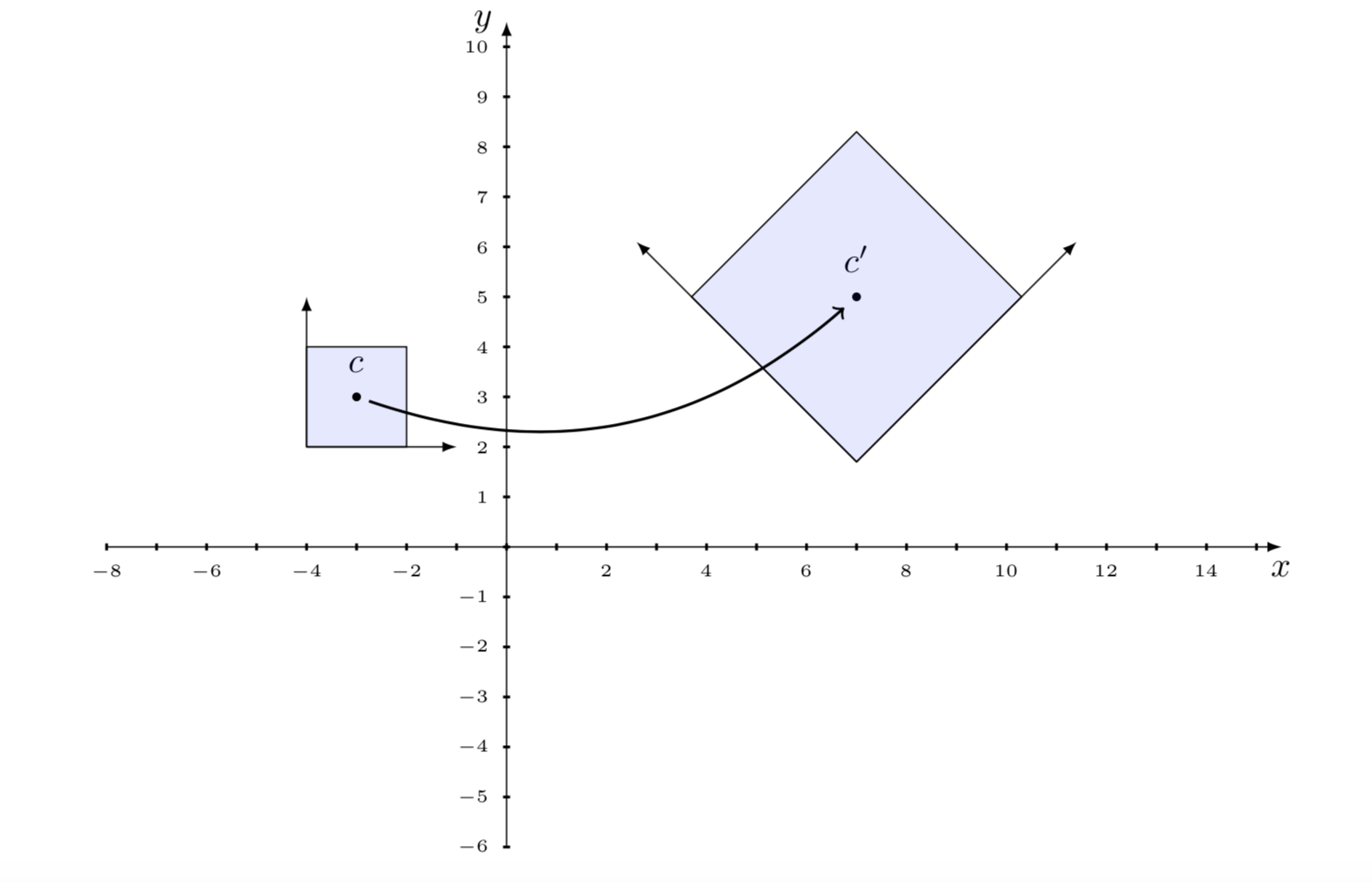
Fractal objects are typically subsets of the Euclidean space \(\mathbb {R^{n}} \), generated by affine transformations. It’s of fundamental importance to study the geometric properties that remain unchanged with respect to an affine transformation.
An affine transformation is a composition of rotations, translations, dilations and contractions. Affine transformations preserve collinearity (i.e. points that initially belong to a straight line, remain on the straight line) and the ratio of distances (midpoint of a line segment remains the midpoint after transformation). However, they do not preserve the angles and lengths.
The affinity relationship is an extension of the congruence and similarity relationships studied in classical Euclidean geometry. A triangle always remains a triangle after an affine transformation, even if it doesn’t necessarily have the same area (congruence) or is similar to the initial one.
To understand the affine transformations it’s necessary to remember the most important properties of the algebra of vectors and matrices. For this you can consult the following text, which proposes many solved exercises: [2]. See also the articles already published in this blog on the topics of algebra of vectors and matrices.
Exercise 5.1
Given an affine transformation \(f (x) = Ax + t \) find the inverse transformation \(g (x) \) such that \(f (g (x)) = x \).
Hint
Multiply left and right by the inverse matrix \(A^{- 1} \).
Theorem 5.1
A composition of two affine transformations is an affine transformation.
Proof
Let \(f (x) = Ax + t \), \(g (x) = Bx + s \) be two affine transformations. Then \((g \circ f) (x) = g(f (x)) = (BA)(x) + (Bt + s) \). Since \(A, B \) are invertible matrices, the product matrix \(BA \) is also invertible, therefore the composite function \(g \circ f \) is an affine transformation.
5.1) Homogeneous coordinates
An affine transformation in the plane can be represented compactly using homogeneous coordinates, that is a matrix \(3 \times 3 \). In fact we add a column with the parameters related to the translation and a row with the values \((0,0,1) \):
\[ Ax + t= \left(\begin{array}{lll} a & b & e\\ c & d & f\\ 0 & 0 & 1 \end{array}\right) \left(\begin{array}{l} x \\ y \\ 1 \end{array}\right) \]For the transformations in the space \(R^{3} \) we will use a matrix \( 4 \times 4 \).
The matrices for the basic transformations are the following:
Translation \((d_{x}, d_{y}) \):
\[ \left(\begin{array}{lll} 1 & 0 & d_{x} \\ 0 & 1 & d_{y}\\ 0 & 0 & 1 \end{array}\right) \]Rotation by an angle \(\theta\):
\[ \left(\begin{array}{lll} \cos \theta & – \sin \theta & 0 \\ \sin \theta & \cos \theta & 0\\ 0 & 0 & 1 \end{array}\right) \]Scaling \((s_{x}, s_{y}) \):
\[ \left(\begin{array}{lll} s_{x} & 0 & 0 \\ 0 & s_{y} & 0\\ 0 & 0 & 1 \end{array}\right) \]Deformation (shear):
\[ \left(\begin{array}{lll} 1 & a_{x} & 0 \\ b_{y} & 1 & 0\\ 0 & 0 & 1 \end{array}\right) \]Example 5.1
The following matrix represents a translation of one unit in the direction of the \(x \) axis and two units in the direction of the \(y \) axis. The dimensions are not changed and there is no rotation.
Exercise 5.2
Determine the effect of the transformation in the plane using the following matrix [\(\cos (30^\circ) = \sqrt \frac{3} {2} ,\sin (30^\circ) = \frac{1} {2} \)]:
6) Transformations in metric spaces
Definition 6.1
Given a metric space \((X, d\) ) and a function \(f: X \to X \), the function is said to be a contraction on the metric space if there exists a real number \(0 \le c <1 \) such that
Definition 6.2
Given a function \(f: X \to X \), a point \(x_{0} \in X \) is called a fixed point for the function if it results \(f (x_{0}) = x_{0} \).
Exercise 6.1
Consider the metric space \((R^{2}, d) \), where \(d \) is the Euclidean metric. Let the transformation \(f: \mathbb{R^{2}} \to \mathbb {R^{2}} \) be given as follows:
Prove under which conditions of the coefficients \(a, b, c \) it’s a contraction and in this case find the fixed point.
Answer: \(\left[ a, c> 1; x = \dfrac{ab} {a-1}, y = \dfrac{bc} {c-1} \right]\)
For contractions the following fundamental theorem of Banach (1892-1945) and Caccioppoli (1904-1959) applies:
Theorem 6.1 – Banach-Caccioppoli
Let \((X, d) \) be a complete metric space and \(f: X \to X \) a function of contraction on the space. Then the function \(f \) has a single fixed point in \(X \). Also, for each point \(x \in X \) the sequence
converges to the fixed point of \(f \).
For the proof see a text of mathematical analysis; for example [3].
Example 6.1
An example of application of this theorem is the search for a solution of the equation \(f (x) = 0 \). First we write the equation in the form \(x = T (x) \), then we define an iteration scheme \(x_ {n + 1} = T (x_{n}) \), starting from an initial value \(x_ {0} \). Under suitable conditions the sequence tends to a fixed point of \(T (x) \), that is to a zero of the function \(f (x) \).
An important example is Newton’s algorithm for finding the roots of a function. Suppose we want to find the solutions of the function \(x^{2} – a = 0 \). We write the equation in the form \(x = \frac{1}{2} (x + \frac {a} {x}) \), and set the iterative scheme:
It can be shown that by appropriately choosing the starting point \(x_ {0} \) the sequence converges to the value \(\sqrt {a} \), which is the fixed point and also the root of the initial equation.
7) Iterated function systems
As we have previously seen, an affine transformation in the Euclidean space \(R^{2}\) which transforms a point \((x_{n}, y_{n}) \) into the point \((x_{n + 1} , y_{n + 1}) \) can be described with the following equations:
\[ \begin{split} x_{n+1} = a x_{n} + by_{n}+ e \\ y_{n+1} = c x_{n} + dy_{n}+ f \\ \end{split} \]The parameters \(a, b, c, d \) produce a rotation and a change of scale according to their size; the parameters \(e, f \) perform a translation of the point. If we take some points of the border of any object, and apply these functions to each of the points, we can obtain a transformation of the whole figure, made of rotations, translations and changes of scale. The new figure will generally have the property of auto-similarity with the original figure, one of the characteristic properties of fractals.
One of the most common ways to generate fractal images is to use an attractor set of an iterated function system (IFS). Each IFS is made up of affine transformations with rotations, translations and changes of scale. Normally two types of algorithms are used, one deterministic and another probabilistic.
For an in-depth study of IFS, see Barnsley’s fundamental text [4].
7.1) Deterministic iterated function systems
Definition 7.1
A deterministic iterated function system (IFS) is a collection of affine transformations \(\{T_{1}, \cdots T_{n} \} \):
The following theorem (see Barnsley) is fundamental:
Theorem 7.1
Let’s consider an iterated function system \(\{H (X); T_{1}, T_{2}, \cdots, T_{n} \} \), with contraction factor \(c \). For each set \(A \in H(X) \) we define the union set
Then:
- \(W(A) \) is a contraction function with factor \(c \)
- there is a single fixed point \(K \in H(X) \) such that \(K = W(K) = \cup T_{i} (K) \)
The fixed point \(K \) is obtained as an infinite limit of the iteration process applied to the set \(A \).
Procedure for creating a fractal with the deterministic IFS method
The deterministic algorithm takes a set of points \(A \), for example the points of a geometric figure, to which it applies the \(n \) affine transformations, thus obtaining a new set consisting of the union of \(n \) sets of points:
\[ W(A)= T_{1}(A) \cup T_{2}(A) \cup \cdots \cup T_{n}(A) \]The operator \(W \) is called the Hutchinson operator.
For example, if the initial set \(A \) consists of only one point, after the first iteration the set \(W (A) \) contains \(n \) points. The iteration process is continued starting from the set \(W (A) \) until the union of all the sets obtained in the last iteration approaches the figure that constitutes the attractor of the IFS system. Each IFS has associated a fractal attractor, which is generally independent of the initial choice of points.
7.2) Random iterated function system
As we mentioned earlier, there is also a nondeterministic version of the IFS algorithm. We define a probability distribution for the various transformations, and at each iteration, instead of applying all the transformations, we choose a transformation based on its probability.
Definition 7.2
A non-deterministic iterated function system is a collection of affine transformations \(\{T_{1}, \cdots T_{n} \} \), associated with a probability distribution \(\{P_{ 1}, \cdots P_{n} \} \):
Instead of applying functions to a set of points, the execution of a random iterated function system begins by choosing an initial point on the plane. Then one of the \(n \) transformations of the system is chosen randomly, based on the individual probabilities of each iteration. This process is repeated theoretically indefinitely. Of course, in practice, when generating the graphic image we stop after a finite number of iterations. After a certain number of iterations, the set of generated points becomes arbitrarily close to the attractor set of the IFS system.
8) The Sierpinski triangle
The Sierpinski triangle (Sierpinski gasket) is a geometric figure proposed by the Polish mathematician W. Sierpinski (1882-1969), which requires the following steps for its construction:
- start with an equilateral triangle, indicated with \(A_{0} \), and identify the midpoints of the three sides
- the three midpoints are connected to each other and the triangle that is created is eliminated, not including its border; the remaining figure is indicated with \(A_{1} \)
- on each of the three remaining triangles the procedure is repeated, obtaining \(A_{2} \), and so on to infinity
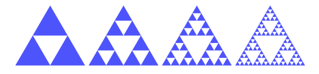
The iterative process creates an infinite succession of sets:
\[ A_{0} \supset A_{1} \supset A_{2} \supset \cdots A_{N} \cdots \]The Sierpinski triangle is the set of points that remain after the procedure is repeated indefinitely.
The initial image is subjected to a set of affine transformations; it’s therefore an iterated function system. In each phase, three blue triangles and a white triangle are created from each blue triangle. Each of the new triangles has the perimeter equal to half of the parent triangle and the area equal to a quarter of that of the parent triangle. The sequence of sets \(\ {A _{0}, A_{1}, A_{2}, \cdots }\) is a sequence of compact sets, since in each step we eliminate the open triangle in the center. After an infinite number of iterations the image converges to the attractor. The system of equations that define the Sierpinski triangle is as follows:
You can also change the procedure, creating a right triangle with three vertices \(\{(0,0), (1,0), (0,1) \} \):
\[ \begin{split} \\ T_{1}(x,y)&= \left(\frac{x}{2}, \frac{y}{2}\right) \\ T_{2}(x,y)&= \left(\frac{x}{2} + \frac{1}{2},\frac{y}{2}\right) \\ T_{3}(x,y)&= \left(\frac{x}{2},\frac{y}{2} + \frac{1}{2}\right) \end{split} \]The functions \(\{T_{1}, T_{2}, T_{3} \} \) are affine transformations, translations and changes of scale. We call \(A_{0} \) the initial image of the triangle with the vertices \((0,0), (1,0), (0,1) \). After the first iteration we get the image
\[ A_{1}= T(A_{0})=T_{1}(A_{0}) \cup T_{2}(A_{0}) \cup T_{3}(A_{0}) \]where the transformation \(T\) is the union of the three elementary transformations. Continuing we have \(A_{2} = T(A_{1}) = T^{2} (A_{0})\), etc. The Sierpinski triangle is the limit of this succession of compact sets:
\[ \text {Sierpinski Triangle} = \lim_{n\to\infty} T^{n}(A_{0}) \]8.1) Area and perimeter of the Sierpinski triangle
To compute the area and the perimeter of the Sierpinski triangle we use the following table:
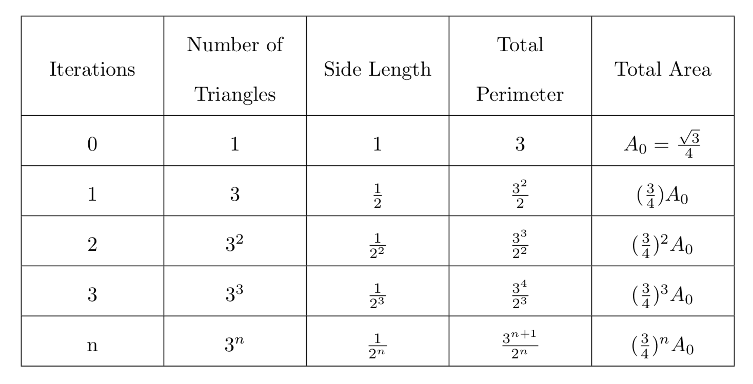
From the table we can conclude that the searched values of the area and the perimeter of Sierpinski triangle are the following:
\[ \begin{split} \text {Perimeter} &= \lim_{n\to\infty} \left(\frac{3^{n+1}}{2^{n}}\right)= \infty \\ \text {Area} &= \lim_{n\to\infty} \left(\frac{3}{4}\right)^{n} \cdot A_{0}=0 \\ \end{split} \]8.2) Dimension of the Sierpinski triangle
In the case of the Sierpinski triangle, at each iteration we have \(N = 3^{n} \) triangles while the length of the sides of the triangles is \(L = \dfrac{1} {2^{n}} \). So, we find the following value for the dimension:
\[ d = \lim_{n\to\infty} \frac{\ln 3^{n}}{\ln 2^{n}} = \frac{\ln 3}{\ln 2} \approx 1,58496 \]The dimension can also be calculated according to another procedure. Since the Sierpinski triangle is self-similar with three disjoint copies of itself, each scaled by the factor \(r = \frac {1}{2} \), the dimension \(d \) of the attractor can be calculated by solving this equation:
\[ r^{d} + r^{d} + r^{d}= 3 \left(\frac{1}{2}\right)^{d}=1 \]For a proof see Barnsley’s book.
Conclusion
As we have seen in this article, fractal science rests on solid foundations, consisting of consolidated sectors of mathematics, such as analysis, topology, geometry, etc. Computer generated fractals are very beautiful and interesting objects attracting many people. However, this is only one aspect; fractal science is also a very important tool for describing complex systems and processes, both natural and artificial.
Bibliography
[1]S. Lipschutz – General Topology (McGraw-Hill)
[2]S. Lipschutz – Schaum’s Outline of Linear Algebra (McGraw Hill)
[3]A. Kolmogorov, S. Fomin – Elements of function theory and functional analysis (Editori Riuniti)
[4]M. Barnsley – Fractals Everywhere (Academic Press)

0 Comments