Euclidean geometry studies geometric objects such as lines, triangles, rectangles, circles, etc. Fractals are also geometric objects; however, they have specific properties that distinguish them and cannot be classified as objects of classical geometry. Although Mandelbrot (1924-2010) is generally considered the father of the scientific theory of fractals, in reality the ideas underlying the theory had been present in various mathematical studies since the previous centuries.
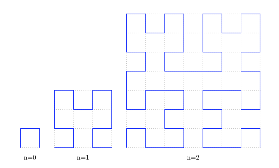
An example of geometric objects that do not fit into the models of classical mathematical analysis are the curves that fill the plane, initially studied by Giuseppe Peano (1858-1932). Among these we illustrate the Hilbert curve (1862-1943), i.e. a continuous fractal curve that fills the whole plane.
1) Properties of the fractals
The concept of fractal is often associated with some properties that distinguish them from the usual geometric objects. These properties include the following:
- self-similarity
- geometric irregularity
- fractional size
1.1) Self-similarity
Self-similarity means that the object is made up of components that have a structure similar to the entire object. Self-similar objects scale by the same amount in each direction. This property of fine structure in the mathematical models of fractals holds at every scale, while in the real world it clearly has limits (due at least to the molecular and atomic structure).
A generalization of self-similarity is self-affinity, i.e. objects that are approximately self-similar at different scales, nevertheless can be different because are scaled by different factors in different directions, with effects of expansion or contraction.
In addition to abstract objects created by mathematics, several examples of fractals are found in nature. Clouds, mountains, coasts, flowers, ice crystals, etc. are all examples of irregular objects that can hardly be described with classical geometry, and have approximate properties of self-similarity.
1.2) Geometrical irregularity
Unlike the curves and surfaces of classical analysis, fractal objects present irregularities at various levels of scale. For example, many fractal curves, while being continuous, do not admit the tangent at any point, therefore it’s not possible to apply the concept of derivative, so important in classical mathematical analysis.
1.3) Fractional dimension
Objects of classical geometry always have integer dimensions equal to:
- \(0\) for the points
- \(1\) for linear figures (straight lines, curves, etc.)
- \(2\) for flat figures (squares, circles, etc.)
- \(3\) for space objects (cubes, spheres, etc.).
In the world of fractals, on the other hand, it is necessary to generalize the concept of dimension, introducing the possibility of fractional values.
To begin the study of fractals, it is necessary to review some concepts of set theory.
2) Basic concepts of Set Theory
A set is a collection of distinct objects, called elements of the set. Objects can be of any nature: numbers, vehicles, people, etc. A set can be defined by describing its content, or by listing the elements that belong to the set.
The universal set is the set that contains all the elements of the context of interest. The empty set does not contain any elements. The complement of a set A is the set which contains all the elements of the universe that do not belong to A.
Given two sets A, B the operations of union and intersection are so defined:
Definition 2.1
Two sets A, B are called equipotent (or have the same cardinality) if there is a biunivocal correspondence between them; that is, if there is a bijective function \(f: A \to B \).
The notion of cardinality of a set was developed by the mathematician Georg Cantor (1845-1918). The cardinality of a finite set is given by the number of elements in the set. Obviously two finite sets are equipotent if and only if they contain the same number of elements. However, for infinite sets the situation is more complex.
Definition 2.2
An infinite set is called countable if it has the same cardinality as the set of natural numbers. Otherwise it is called uncountable.
Exercise 2.1
Prove that all the following sets are countable, finding for each set a bijective function with the set of natural numbers:
- \(\mathbb{N} \) – natural numbers \( \{1,2,3, \cdots \}\)
- \(A\) – even positive integers \( \{2,4,6, \cdots \} \)
- \(B\) – odd positive integers \( \{1,3,5, \cdots \} \)
- \(\mathbb{Z}\) – integers \(\{\cdots ,-3,-2,-1,0,1,2,3, \cdots \}\)
It can be shown that also the set of rational numbers is countable.
Cantor’s fundamental discovery is that the set of real numbers (which includes the rational and irrational) is not countable. We say that the set of real numbers has the power of the continuum.
Theorem 2.1 – Cantor
The set of real numbers is not countable.
Proof
In reality it is sufficient to show that the set of real numbers contained in the interval \([0,1]\) is uncountable. We use the famous Cantor’s diagonal procedure.
Suppose it is possible to establish a one-to-one correspondence between the set of natural numbers and the interval \([0,1]\), that is there is a bijective function \( f: \mathbb{N} \to [0,1]\). We list this correspondence through the binary expansion of the real numbers included in the interval \([0,1]\):
where \(a_{ij}\) take the values \(\{0,1\}\). Cantor’s diagonal procedure consists of determining a real number in the interval \([0,1]\) that is different from all the numbers \(f(i)\). The number searched has the following binary expansion: \(x=0.b_{1}b_{2}b_{3} \cdots \), where the digits are defined as follows:
\[ \begin{cases} b_{k}= 0 \quad if \quad a_{kk}=1 \\ b_{k}= 1 \quad if \quad a_{kk}=0 \end{cases} \]It is evident that for no value of \(n\) one has \(f(n)=x\), then the function is not bijective, which is contrary to the hypothesis.
Exercise 2.2
Show that the interval \((0,1)\) and the infinite line \((-\infty,+\infty)\) have the same cardinality.
Hint
Use one of the trigonometric functions to find a one-to-one correspondence between the two sets.
Here we conclude these references to set theory. For a review of the elementary set theory, with several solved exercises, see for example [1].
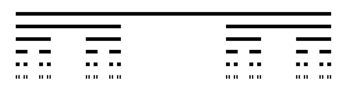
3) Cantor set
The Cantor set is another famous example of sets that do not fit into the models of Euclidean geometry and classical mathematical analysis.
The construction of the Cantor set is based on a simple iterative process. A unitary segment \([0,1]\) is taken and the central segment \((\frac{1}{3},\frac{2}{3})\) is removed, leaving the extreme points. Then the same procedure is repeated on each of the two remaining segments, and so on ad infinitum.
The Cantor set consists of all the points in the interval \([0,1]\) which are not eliminated in this infinite process of cancellation.
A first interesting thing is to compute the overall length of the deleted segments:
\[ L=\frac{1}{3} + 2 \frac{1}{3^{2}} + 2^{2} \frac{1}{3^{3}}+ \cdots = \frac{1}{3} \sum_{k=0}^{\infty} \frac{2^{k}}{3^{k}}=1 \]as it is a geometric series. Remember that for a geometric series we have
\[ \sum_{k=0}^\infty x^{k}= \frac{1}{1-x} \quad if \quad |x| <1 \]At first sight it would it seems that the cutting process eliminates all points and nothing remains of the initial segment, but it isn’t so; in fact, having preserved the extreme points of the segments, they are never eliminated. For example, the point \(\frac{2}{3}\) of the first iteration is left and there will be no more segments containing it. To understand exactly which and how many points in the interval \([0,1]\) remain at the end of the iterative process, it is convenient to express the real numbers of the interval with the ternary system.
3.1) The ternary system
The decimal system uses the symbols \(\{0,1,\cdots,9\} \); for example, the number \(25\) in the decimal \(25_{10}\) is equivalent to
\[ 25_{10}= 2 \cdot 10^{1}+ 5 \cdot 10 ^{0} \]The ternary system uses the symbols \(\{0,1,2 \}\) to represent a real number. The number \(221_{3}\) in base \(3\) is equivalent to
\[ 221_{3}=2 \cdot 3^{2} + 2 \cdot 3^{1}+ 1 \cdot 3^{0}=25_{10} \]The fractional number \(21,011_{3}\) is equivalent to
\[ 2 \cdot 3^{1} + 2 \cdot 3^{0}+ 0 \cdot 3^{-1} + 1 \cdot 3^{-2} + 1 \cdot 3^{-3} \]The representation of numbers with the ternary system helps us to understand what happens in the iterative process of deleting segments of the Cantor set described above.
In the first iteration the central segment \((\frac{1}{3},\frac{2}{3})\) is removed. In fact we remove the numbers which, in base \(3\), have the digits equal to \(1\) in the first position.
In the second iteration the central range is removed in each of the two segments \([0,\frac{1}{3}]\), \([\frac{2}{3},1]\). In each of the two intervals we remove the numbers which, in base \(3\), have the digits equal to \(1\) in the second position.
Continuing to infinity we can conclude that the Cantor set contains all the real numbers whose ternary expansion contains only the digits \(\{0,2\}\). So the Cantor set is not empty, as it might have seemed at first sight, but it contains infinite points. Indeed the following theorem can be proved:
Theorem 3.1
The Cantor set is not countable, but has the same power as the set of all real numbers (continuum power).
For a proof see the text quoted above.
4) The dimension of fractal
Fractal objects, although they can be represented in a geometric space of 1,2,3 dimensions, do not have an integer dimension. The dimension of a fractal object gives a measure of how complicated a self-similar figure is, of how many points lie in a given set.
There are different definitions of size; in this article we will describe the box-counting procedure, which is the simplest and most intuitive and is still sufficient to study most fractal objects.
To understand the motivation behind the box-counting procedure, let us take for example a square, which has a dimension equal to \(2\); dividing the sides in half we get \(2^{2}=4\) squares with sides equal to \(\frac{1}{2}\) of the original ones; if we divide the initial square into squares of side \(\frac{1}{3}\) we obtain \(3^{2}=9\) squares with sides equal to \(\frac{1}{3}\) of the initial ones. Continuing like this, we can deduce an important relationship between the number of produced squares \(N\), the scale factor \(f\) and the size of the objects \(D\). The formula is the following:
Calculating the natural logarithm we obtain the following relations:
\[ \begin{array}{l} \ln N = D \ln \dfrac{1}{f}= \ – D \ln f \\ D= -\dfrac{\ln N}{\ln f} \end{array} \]Definition 4.1 – Box-Counting dimension
We give the definition of dimension of a bounded fractal object contained in the Euclidean space.
Let \(N(S,d)\) be the number of small cubes with side \(d\) necessary to cover the object \(S\). Every object \(N(S,d)\) therefore contains at least one point of \(S\). The idea is to take cubes with smaller and smaller sides and define the dimension of S as the limit of the following expression:
In the case of flat objects we use squares, instead of cubes. For objects contained on a line, segments are used. Of course this definition only makes sense if the limit exists. In mathematics there are more advanced definitions, such as the Hausdorff-Besicovitch dimension, which does not give different results from box-counting in the most common cases though. For a more advanced study you can consult the text [2].
For the objects of Euclidean geometry, the fractal dimension coincides with the classical dimension.
Example 4.1 – Dimension of the square
It is given a square Q of unitary side. In this case, if we set \(d=\frac{1}{n}\) we have \(N\left(Q,\frac{1}{n}\right)= \frac{1}{n^{2}}\). Applying the formula, we find:
With the same method, we find that the cube has dimension equal to 3.
Example 4.2 – Fractal dimension of the Cantor set
Based on the iteration process, we can compute the number of components for each value of n:
Applying the definition, we have:
\[ \text {dim(S)} = \lim\limits_{n \to \infty} \frac {\ln(2^{n})}{\ln(3^{n})}=\frac {\ln(2)}{\ln (3)} \approx 0.631 \\ \]5) The Koch curve and the snowflake
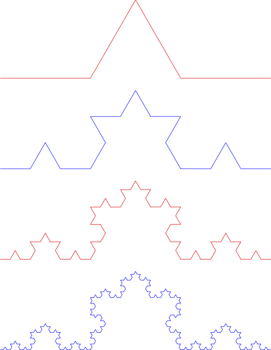
The snowflake by Von Koch (1870-1924) is a curve constructed by working on the sides of an equilateral triangle. On each of the sides of the triangle the Koch curve (also called the Koch lace) is built: take the side, cut it into \(3\) parts and replace the central one with two segments equal to the one eliminated; the operation is repeated with each of the four segments thus obtained and is continued for an infinite number of times. The figure obtained operating on three sides, after an infinite number of iterations, is Koch’s snowflake.
Von Koch’s lace is clearly self-similar, while the snowflake is not strictly self-similar. In fact, by enlarging one of the sides after the first iteration we get a copy of the lace and not of the entire snowflake.
It can be shown that the Koch curve is continuous at every point, but it is not derivable at any point. The following image illustrates the first 3 iterations of the process of dividing a side of the triangle.
5.1) Length of the Koch curve and the snowflake
At each iteration the length of the Koch curve increases by a factor \(\frac{4}{3}\): if the starting segment has length equal to \(1\), the second measures \(\frac{4}{3}\), the third \(\frac{16}{9}\), the fourth \(\frac{64}{27}\) and so on. So at the step \(n\) of the construction process we have \(4^{n}\) segments, each of length \(\frac{1}{3^{n}}\). The total length \((\frac{4}{3})^{n}\) tends to an infinite value. Therefore we can conclude that the perimeter of the Koch curve and consequently also of the flake has an infinite value, even though the two curves are contained in a bounded region.
5.2) Fractal dimension of the Koch curve
At each iteration step, each segment of the Koch curve is replaced by 4 small segments, each of length equal to \(\frac{1}{3}\) of the initial one. So applying the definition of fractal dimension, we have:
\[ \text {dim(K)} = \lim\limits_{n \to \infty} \frac {\ln(4^{n})}{\ln(3^{n})}=\frac {\ln(4)}{\ln (3)}= \approx 1.262 \]5.3) Koch snowflake area
Suppose the equilateral triangle has unitary sides. The area is therefore \(\frac{\sqrt{3}}{4}\). The first iteration adds 3 triangles. Each of the following iterations adds a number of triangles 4 times the previous one. Then the n-th iteration adds \(3 \cdot 4^{n-1}\) triangles. We can write the following recursion equation for the area of the figure:
\[ A_{n}= A_{n-1}+ \frac {3 \cdot 4^{n-1}}{9^{n}} A_{0} \]where \(A_{0}\) is the area of the initial triangle. It’s a recurrence equation that can be solved with the methods of finite difference equations (for which we refer to the text [3]). However in this case the equation is quite simple and with a few elementary steps we can calculate the area of the Koch snowflake:
\[ A = \lim_{n \to \infty} A_{n}= A_{0} \lim_{n \to \infty} \left[1+ \frac{1}{3}\sum_{k=0}^{n-1}\left(\frac{4}{9}\right)^{k}\right]= \frac{8}{5}A_{0} \]where we used the sum of the geometric series.
6) Fractals and chaotic systems
The scientific and technological development that characterizes the modern age is based on the application of mathematics to various disciplines. Mathematical tools have allowed in the last few centuries to predict and compute the evolution of physical phenomena with great precision, especially in the case these are determined by linear laws. However, despite the availability of more and more powerful computers, a lot of them remain outside the possibility of a reliable forecast. The problem is that many physical, economic and social phenomena have a chaotic and non-linear nature, which prevents them from reliably predicting future behaviour. Several natural or artificial systems such as economies, stock markets, chemical reactions, etc. show a great dependence on initial conditions. Even small differences in initial conditions can lead to big differences in future evolution. Moreover, the initial conditions are never known with absolute precision and mathematical and physical models are always approximations of real phenomena. In this situation, any reliable long-term future forecast is almost impossible.
The chaotic aspect of the behaviour of all physics systems subject to non-linear forces was recognized by the great french mathematician H. Poincaré (1854-1912), in his work “Science and Method”, with these words: “It may happen that small differences in the initial conditions produce very great ones in the final phenomena. A small error in the former will produce an enormous error in the latter. Prediction becomes impossible, and we have the fortuitous phenomenon”.
Fractals are often used to model chaotic processes, which despite having an apparently random behavior, present characteristics of self-similarity in detail.
The science of fractals therefore consists not only in complex graphic images generated by computers, but provides tools that allow the creation of models of complex phenomena, with precision in some cases greater than traditional models of classical mathematics and physics.
Conclusion
The science of fractals and chaotic systems integrates different disciplines, such as mathematics, physics and computer graphics. It’s a real scientific revolution that will allow us to make important progress in the search for increasingly precise models to study both complex mathematical objects and the evolution of real world phenomena. For a serious study of fractals, you can consult the following books [4] and [5].
Bibliography
[1]Lipschutz – Set Theory and Related Topics (McGraw-Hill)
[2]M. Barnsley – Fractals EveryWhere (Dover Books)
[3]M. Spiegel – Differenze finite e equazioni alle differenze (Etas Libri)
[4]Mandelbrot – The Fractal Geometry of Nature: Set Theory and Related Topics (Times Books)
[5]Falconer – Fractal Geometry (Wiley)

0 Comments