The study of integers and their properties is the fundamental object of Number Theory. The properties of prime numbers and divisors of an integer were first studied extensively during the period of ancient Greece (Pythagoras, Euclid, etc.); the study resumed again in the seventeenth century, in particular thanks to the contributions of Fermat, and then continued in the following centuries.
Let’s introduce some definitions of the various types of sets that are studied in Number Theory:
- the set \( \mathbf{P}\) of prime numbers, that is \( \mathbf{P}= \{2,3,5,7,11,13,17,…..\}\);
- the set of positive integers, or natural numbers, indicated with \( \mathbf{N} \), that is \( \mathbf{N}=\{1,2,3,4,…\} \);
- the set \( \mathbf{Z} \) of integers, that is \( \mathbf{Z}= \{…,-4,-3,-2,-1,0,1,2,3,4,…\}\);
- the set of rational numbers \( \mathbf{Q} \), defined as \( \mathbf{Q} = \{\frac {a} {b}; a,b\in \mathbf{Z};b \ne 0\}\);
- the set of real numbers \( \mathbf{R} \), which includes the rational and irrational numbers; every irrational number is limit of a sequence of rational numbers;
- the set of complex numbers \( \mathbf{C} \); each complex number is an ordered pair of real numbers.
A prime number is an integer greater than \(1\) which is divisible only by \(1\) and by itself. An integer that is not prime is said to be composite. Prime numbers are the building blocks of integer numbers, thanks to the fundamental theorem of arithmetic, which states that every positive integer can be expressed in a unique way as a product of powers of prime numbers. To determine the factorization of a positive integer n you can use the function n.factor() in the SageMathCell environment. For example 588.factor() give the result \( 2^2 \cdot 3 \cdot7^2 \).
1) Arithmetic functions
An arithmetic function is a function \( f(n) \) which assigns a real or complex number to each natural number. In symbols
\[ f\colon N \to C,\quad n \mapsto f(n) \]An arithmetic function \( f(n) \) is said to be multiplicative if
\[ f(ab)=f(a)f(b) \]for all pairs of positive integers \( a,b\in\mathbf{N} \) such that \( (a,b)=1 \). (The symbol \( (a, b) \) represents the greatest common divisor of the two numbers).
An arithmetic function \( f(n) \) is said to be completely multiplicative if \( f(ab)=f(a)f(b)\) for all pairs of positive integers \( a,b \).
Theorem 1.1
Let \( f(n) \) be a multiplicative function. Then
This property follows directly from the definition.
Theorem 1.2
If \( f(n) \) is a multiplicative function, then also the following function:
is multiplicative. For a proof see [1].
2) The number of divisors of an integer
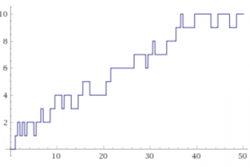
As a first example of an arithmetic function, we introduce the function \( d(n) \), whose value is given by the number of divisors of \( n \). If \( n \) is a prime number then \( d(n)=2 \) , as the only divisors are \( 1,n \).
For a composite number the function \( d(n) \) is easily computed starting from the factorization in prime factors.
For example if \( n=p^{k} \) then the divisors are \( \{1,p,..p^{k-1}, p^{k}\} \), and therefore \( d(p^{k})=k+1 \) .
If \( n=p_1^{a_1}p_2^{a_2} \) then the divisors are all numbers of the type \( p_1^{b_1}p_2^{b_2} \), where \( 0 \le b_1 \le a_1 \) and \( 0 \le b_2 \le a_2 \). So the total number of divisors is given by the product \( (a_1 + 1)(a_2 + 1) \) . In general we have the following formula:
This result could be obtained by observing that \( d(n)=\sum_{d\mid n}1 \), the function defined \(f(n)=1 \) for all values of \(n \) is multiplicative and therefore by the Theorem 1.2 also the function \( d(n) \) is multiplicative.
To determine the list of divisors of a number n we can use the n.divisors() function of the SageMathCell program. For example 999.divisors() results in the list \( [1, 3, 9, 27, 37, 111, 333, 999] \).
Exercise 2.1
Given a positive integer \( m \), find all the integers \( n \) for which \(d(n) = m\).
Hint
Use the Rule of John Wallis (1685). Find all possible factorizations of \( m \); if the factors are \( a, b, … \) then the required number is \( p^{a-1} q^{b-1}… \), where \( p, q, …\) are distinct prime numbers at will.
As an example, determine the natural numbers \( n\) such that \(d(n)=10 \) .
Exercise 2.2
Prove that, given \( n >1 \) , the sequence of the following numbers from a certain point onwards takes on the constant value \( 2 \):
The point can be moved forward as desired, using \(2^{n-1} \) as initial value.
3) The product of the divisors of an integer
To compute the product of all divisors of \(n\), it is enough to observe that the divisors can be grouped in pairs: for each divisor \(d \), we have the unique complementary divisor \(\delta = \frac{n}{d}\), as \(n = d \delta \). If \(d \) varies on all possible divisors of \(n \) , then it is obvious that \( \delta \) assumes the same set of values. Putting together we have:
\[ \begin{array}{l} \prod\limits_{d \mid n} d = \prod\limits_{\delta \mid n}\delta \\ \\ n^{d(n)} = (\prod\limits_{d\mid n}d) (\prod\limits_{\delta \mid n} \delta)=(\prod\limits_{d\mid n}d)^2 =\prod\limits_{d\mid n}d^2 \end{array} \]So we have the following result:
Theorem 3.1
The product of the divisors of an integer \( n \) is
4) The sum of the divisors of an integer
The sum of positive divisors is defined as
\[ \sigma (n) =\sum\limits_{d\mid n}d \]For example \( \sigma (12) = 28 \). We note that \( \sigma (4) = 7\) and \( \sigma(3)=4 \). Then \( \sigma(12) = \sigma(4) \cdot \sigma(3) \). This is a general result as the function \( \sigma (n)\) is multiplicative.
Theorem 4.1
The function \( \sigma (n) \) is multiplicative.
Proof
To prove it, just use the theorem 1.2 with the function \( f(n)=n \).
The value of \( \sigma(n) \) is therefore completely determined if we know the values on the powers of the primes. If \( p \) is a prime number and \(a \) is a positive integer then:
\[ \sigma(p^a)= 1+p+…+ p^{a}= \frac{p^{a+1}-1}{p-1} \]being the sum of a geometric progression.
In general if \( n=p_1^{a_1}p_2^{a_2}…p_k^{a_k} \) we have
Example 4.1
\[ \sigma(300)=\sigma((2^2)(3)(5^2))=\frac{2^3-1}{2-1} \frac{3^2-1}{3-1}\frac{5^3-1}{5-1}=868 \]To check the calculations, type sum(divisors (300)) in the SageMathCell environment.
Exercise 4.1
Show that there is no natural number \( n \) such that \( \sigma(n)=5 \) .
Theorem 4.2
There are infinite natural numbers \( m \) for which the equation \( \sigma(n)=m \).
For a proof see [2].
Exercise 4.2
Prove that if \( \sigma (n) \) is prime, then also \( d (n) \) is prime.
Check if the opposite is true?
Proof
It is obvious that the factorization of \( n \) must be \( n=p^{a} \) as the function \( \sigma (n) \) is multiplicative. Then \( \sigma (n) = 1 + p + …p^{a}= \frac {p^{a+1} – 1}{p-1}=q \) where \( q \) is prime. The exponent \(a\) must be even and \( a+1 \) must be prime, otherwise \(q \) would not be prime. Then also \( d(n)= a+1 \) is prime.
Clearly the reverse is not true; for example \( d(49)=3 \), while \( \sigma (49) = 1+7+49 = 57 = 19 \cdot 3 \) .
Exercise 4.3
Determine for which integers \( n \) we have \( \sigma (n) = m^2 \).
Hint
An empirical method is the following: let us say \( n=p\cdot m \) where \(p \) is a prime number and \( (p,m)=1 \). Since \( \sigma (pm)= (p+1)\sigma(m)= t^{2} \), it must be \( p= \frac {t^{2} – \sigma(m)}{\sigma(m)} \).
For example if \( t=12\) and \( \sigma(m)=3\) we have \( p = 47 \); as \( \sigma(2) = 3 \) we have \( \sigma (47 \cdot 2)= 48 \cdot 3 = 144 = 12^{2}\).
Theorem 4.3
There are infinite numbers \( n \) such that \( \sigma(n) = m^2\) .
For a proof see [3].
5) The additive functions \( \omega (n)\) and \( \Omega(n)\)
Remember that an arithmetic function is called completely additive if
\[ f(nm)=f(n)+ f(m) \]for each pair of integers \( n,m \in \mathbb{N} \).
If the relation is valid only for the pairs of prime integers among them, that is if \( (n,m)=1 \), then the function is called additive.
The function \( \log(n) \) is a completely additive function, as is known that \(\log(nm) = \log(n) + \log(m) \).
An example of additive arithmetic function is the function \( \omega (n)\) defined as the number of distinct prime numbers divisors of \( n\).
Another example of a completely additive function is given by the function \( \Omega (n) \) defined as the number of powers of prime numbers divisors of \( n\).
In symbols if \( n=p_1^{a_1}p_2^{a_2}…p_k^{a_k} \) then
Clearly for an additive function \( f(n) \) it must be \( f(1) = 0 \).
6) Perfect numbers
A positive integer \( n \) it’s called perfect if
\[ \sigma(n)=2n \]that is if the sum of all the divisors (including itself) is twice the number itself. It’s called defective if \( \sigma (n) < 2n \) and abundant if \(\sigma (n) >2 n \).
Examples of perfect numbers, that were already known to the ancient Greeks, are the numbers 6 and 28. To check perfect numbers we use the following theorem.
Theorem 6.1
An even positive integer \( n \) is perfect if and only if
where \( k \) is an integer such that \( k\ge 1 \) and \( 2^{k+1} -1 \) is a prime number. The numbers of the type \( n=2^{k}(2^{k+1}-1) \) are called Euclidean numbers.
For a complete proof see [4]. We only prove that the condition is sufficient. First of all we have
We note that \( \sigma(2^{k})=(2^{k+1}-1) \) and because \( 2^{k+1}-1 \) is prime by hypothesis we have \( \sigma(2^{k+1}-1)=2^{k+1} \). Then
\[ \sigma(n)= (2^{k+1}-1)2^{k+1}= 2n \]Exercise 6.1
Prove that every even perfect number ends with the digit 6 or 8.
Hint
In the formula \( n=(2^{k})(2^{k+1}-1) \) the number \( p=k+1 \) must be prime (see theorem in the paragraph on Mersenne numbers). Then analyse the following cases: \( p = 2, p = 4m + 1, p = 4m + 3 \).
At present no perfect odd numbers are known. However, if they exist, they must be very large. In 1888 Catalan showed that if there is an odd perfect number without the factors (3,5,7) then it must have at least 26 prime factors. In 1953 Touchard showed that a perfect odd number must be of the form \( 12k + 1 \) or \(36k + 9 \). Modern computers have allowed us to exclude the existence of perfect odd numbers with less than \( 300 \) digits, that is, less than \( 10^{300} \).
7) Amicable numbers
We can also define the function
\[ s(n) = \sigma(n) – n \]that is \(s(n)\) is the sum of the proper divisors of \( n \). The Greek mathematician Pythagoras of Samos was among the first ones to observe that \( s(220) = 284, s(284) = 220 \).
We call two numbers \( n,m \) amicable if \( s(n) = m, s(m) = n \).
Exercise 7.1
Prove that if two numbers \(m,n \) are amicable then \(\sigma(n) = \sigma(m)\).
Although many pairs of amicable numbers have been found, the problem of establishing whether there is an infinite number remains open. For the state of the art on amicable numbers see the site Amicable Numbers.
8) Mersenne numbers
The study of perfect numbers leads to the definition of the so called Mersenne numbers (1588 – 1648). Given a positive integer \( k \), the number
\[ M_{k}=2^{k}-1 \]is called Mersenne number . If \( M_{k} \) is prime, then \( M_{k} \) is called a Mersenne prime.
Example 8.1
\(M_3=2^3-1=7\) is a Mersenne prime.
A necessary condition for \(M_{k}\) to be prime is given by the following theorem.
Theorem 8.1
If \(M_{k}=2^{k}-1\) is a prime number, then \(k\) is prime.
Proof
For the proof use the following identity: if \( m = rs \), then
The converse is not true. For example
\[ M_{11}=2^{11}-1=2047=23 \cdot 89 \]Mersenne made the conjecture that \( M_{n} \) is prime for the following values of \( n= 2, 3, 5, 7, 13, 17, 19, 31, 67, 127,257 \) and it is composite for all the other integers \(n \le 257 \). The conjecture was incorrect; the exact list of the first Mersenne primes is the following:
\[ n = 2, 3, 5, 7, 13, 17, 19, 31, 61, 89, 107, 127 \]The largest Mersenne prime number known to 2017 is \( 2^{77,232,917} – 1 \), a huge number of \( 23,249,425 \) digits. See the GIMPS website.
The following theorem is useful to find possible prime divisors of a Mersenne number.
Theorem 8.2
The prime numbers \(q \) which divide \( M_p=2^p-1 \), with \(p \in \mathbb{P}\), are of the form \( q=kp+1 \), where \( k \in \mathbb{N} \).
For a proof see [5].
Exercise 8.1
Use the previous theorem to prove that \( M_{11} \text { and } M_{23} \) are not primes.
Hint
Try the potential divisors up to the value \( \sqrt{M_{n}} \)).
The conjecture that infinite Mersenne primes exist is yet to be proven.
9) Fermat numbers
The integers of the form
\[ F_n=2^{2^n}+1 \]are called Fermat numbers (Pierre Fermat, 1607-1665).
Exercise 9.1
Prove that in order for the number \( F_{n} \) to be prime, it is necessary that \( n \) does not contain odd divisors.
Hint
Remember the following special product, valid when \(b\) is odd:
In the search for possible prime numbers, we can set \( n=2^{k} \). By performing the calculation Fermat found the following values:
\[ F_0=3 , F_1=5 , F_2=17 , F_3=257, F_4=65,537 \]i.e. the first \( 5 \) are prime numbers. This led Fermat to conjecture that all Fermat numbers are prime. However Euler managed to compute \( F_5 \) proving that it is composite:
\[ F_{5} = 4294967296+1=4294967297=641 \cdot 6700417 \]Fermat’s conjecture was therefore wrong. Actually all the numbers of Fermat with \(n < 31 \) are composite. The computation of \( F_{5} \) is very difficult without a computer. However Euler was able to compute it thanks to the following property that he himself proved.
Theorem 9.1
Each divisor of a Fermat number \( F_{n} \) with \( n >2 \) has the shape \( k2^{n+1}+1 \), with \(k \in \mathbb{N}\).
For a proof see [6].
In case \( n=5 \) therefore the prime factors have the form \( p=64k+1 \). With few steps we find the prime numbers \( \{193,257,449,577,641 \} \), the last of which is a divisor of \( F_{5} \).
At present the first \( 12 \) numbers of Fermat have been factored. Two fundamental unresolved problems are the following:
- are there infinite many Fermat primes?
- are there infinite many composite Fermat numbers?
The prevailing opinion is that there are only a finite number of Fermat prime numbers.
Theorem 9.2
For every positive integer \(n \), we have
The theorem is easily proved by induction.
Thanks to the previous theorem we can prove the following property of Fermat numbers:
Theorem 9.3
Let \( r \neq s \) be two non-negative integers. Then \( (F_r,F_s)=1\).
Proof
Suppose \(r<s \). Then \( F_0F_1F_2…F_r…F_{s-1}=F_s-2 \). If by absurd there exists a common divisor \( d \) of \( F_r \) and \(F_s \), then \(d \) should also divide \( F_s-F_0F_1F_2…F_s…F_{s-1}=2 \), which shows that the possible values are \( d=1 \text{ or } d=2 \). But \(F_s\) is always odd and therefore \( d=1 \).
Thanks to the previous theorem it is possible to give further proof of the fact that infinite primes exist (the first proof was given by Euclid in the Elements).
Theorem 9.4 – Goldbach
There are infinite prime numbers.
Proof
Every Fermat number \( F_{n} \) has at least one prime factor \(p_{n} \). These are all different and therefore must be infinite, given that the \( F_{n} \) are infinite.
Exercise 9.2
Using the previous theorem, prove the following estimate for the function \( \pi(x)\), which counts the number of primes \( \le x \):
Fermat’s numbers play an important role in solving a geometric problem that had interested mathematicians since ancient times: can we construct a regular polygon using only a compass and a ruler? The fundamental result proved by Gauss is the following.
Theorem 9.5 – Gauss
A regular polygon of \( n \) sides can be constructed with ruler and compass if and only if
where \( t,k \) are non-negative integers e \( p_{1},…p_{k} \) are Fermat’s prime numbers. For a proof see [7].
10) Relationship of \( \sigma(n) \) with Riemann’s hypothesis
The Riemann zeta function \( \zeta(s) \) is an analytic function that has a fundamental role in the theory of numbers. A definition is as follows:
\[ \zeta(s)=\sum\limits_{n=1}^{\infty}\frac{1}{n^s} \]where \( s = \sigma + it \), with \(\sigma, t \in \mathbb{R}\) and \( i \) is the imaginary unity such that \( i^{2}=-1 \). The series converges if \( \sigma >1 \). The extension to the whole complex plan defines an analytical function in the whole plan, excluding the point \( s=1 \), in which the function has a pole and becomes of infinite module.
The connection of the zeta function with the prime numbers is given by the following Euler product formula:
where \( \{p_n\} \) is the sequence of prime numbers. For a proof see[8].
Exercise 10.1
Use Euler’s product formula to prove that the number of primes is infinite.
Hint
Remember that the harmonic series \( \sum\limits_{k=1}^{\infty} \frac{1}{k} \) is divergent.
Riemann’s hypothesis states that, with the exception of trivial zeros \( s \in \{-2,-4, -6, \text{etc.}\}\), all other zeros of the zeta function are in the line \( \sigma =\frac{1}{2}\).
Now let’s define the function
where \( \gamma \) is the Euler constant, an irrational number whose approximate value is \( \gamma \approx 0.57721 \). The following result can be proved:
Theorem 10.1 – Robin, 1984
The Riemann hypothesis is true if and only if \(f(n) \le 1 \text { for all } n \ge 5041\).
For a proof see Robin’s Criterion.
The Riemann hypothesis has not yet been proved, despite the efforts of the best mathematicians. In 1914 the English mathematician Hardy showed that there are infinite zeroes on the critical line \( \sigma = \frac{1}{2} \). In 1974 Levinson showed that more than one third of the zeros of the zeta function are on the critical line. Despite these important results, the probability of proving the Riemann hypothesis still seems very remote.
Bibliography
[1]Niven, Zuckerman, Montgomery – An introduction to the Theory of Numbers, V edition (Wiley, 1991), pag. 190
[2]Sierpinski – Elementary Theory of Numbers (North-Holland Mathematical Library, 1988)
[3]The American Mathematical Monthly, Vol. 119, No. 5 (May 2012), pp. 373-380
[4]Hardy-Wright – An introduction to the Theory of Numbers, V edition (Oxford, 1979), pag. 239,240
[5]Everest, An introduction to Number Theory- (Springer GTM, 2005), pag. 25
[6]Everest, An introduction to Number Theory- (Springer GTM, 2005), pag. 30
[7]Stewart – Galois Theory, II edition (Chapmann & Hall, 1989; Oxford, 1979), pag. 169
[8]Niven, Zuckerman, Montgomery – An introduction to the Theory of Numbers, V edition (Wiley, 1991), pag. 381

0 Comments